QTT and the Nonlinear Calcium King Plot: Why the Effect Is Expected (and How to Compute It)

A recent high-precision study of isotope shifts in Ca⁺ and highly charged Ca¹⁴⁺ reported a statistically significant nonlinearity in the King plot. After subtracting the small second-order mass shift, the remaining curvature matches what is expected from Standard-Model nuclear polarization. The same dataset is then used to set strong bounds on any new short-range electron–neutron force. (Phys. Rev. Lett. 134, 233002 (2025))

This post explains, in clear and rigorous terms, why this outcome is exactly what Quantum Traction Theory (QTT) https://doi.org/10.5281/zenodo.17594186 predicts natively, how QTT computes the curvature, and why the standard two-parameter King linearity is broken by a parameter-free nuclear–polarization functional.

One-Line Intuition (Plain Language)

In QTT, the electromagnetic response of electrons is fixed universally by a single spectral kernel — no hidden knobs, no per-transition tuning, no extra low-energy forces. Therefore any King-plot curvature must come entirely from the nucleus, not from electronic adjustments and not from a new Yukawa interaction. This is exactly what the Ca/Ca¹⁴⁺ data show.

---

1. From Leading-Order King Linearity to QTT’s Curvature Term

For a transition i between isotopes A and A′, the usual (leading-order) isotope-shift form is:

δνᵢ(AA′) = Kᵢ μ(AA′) + Fᵢ Δ⟨r²⟩(AA′) + Δᵢ(AA′)

If Δᵢ vanished (or factorized), two transitions would form a perfectly straight King plot. But Δᵢ contains higher-order Standard-Model pieces — especially nuclear polarization — which break that linearity.

QTT’s Electromagnetic Universality Postulate

QTT replaces ad-hoc atomic structure corrections with a single universal kernel Kᵢ(ω) fixed once.

Quantum Traction Theory and the Nonlinear Calcium King Plot

In 2025, a beautiful precision experiment on calcium isotopes made headlines in the precision-physics community: they measured isotope shifts in Ca⁺ and highly charged Ca¹⁴⁺, found a strong nonlinearity in the King plot, and then used that nonlinearity to set very strong limits on new short-range forces between electrons and neutrons. The paper is: Phys. Rev. Lett. 134, 233002 (2025) .

From the point of view of Quantum Traction Theory (QTT), this entire story is not a surprise. In fact, the effect is exactly what QTT predicts in the atomic regime: King-plot curvature coming purely from Standard-Model nuclear polarization filtered through a universal electronic kernel, with no need for a new light boson at these energies.

---

1. King Plots 101: Why They Are Linear (and When They Bend)

Consider an electronic transition i and two nuclear isotopes with mass numbers A and A′. The transition frequency shifts by an amount

δνiAA′ = Ki μAA′ + Fi δ⟨r²⟩AA′ + ΔiAA′.

• μAA′ = 1/MA − 1/MA′ is the reduced mass factor.
• Ki and Fi are electronic factors for the mass and field (charge-radius) shifts.
• ΔiAA′ collects all higher-order corrections (second-order mass shift, nuclear polarization, etc.).

If ΔiAA′ were negligible or factorized with the same two nuclear parameters (μ and δ⟨r²⟩) for any transition, then plotting isotope shifts for transition i against those for transition j would yield a perfectly straight line: a King plot.

In practice, higher-order Standard-Model terms (especially nuclear polarization) introduce small, transition-dependent corrections. These break the simple two-parameter factorization and result in an observable curvature in the King plot.

---

2. The QTT View: One Universal Electronic Kernel + Nuclear Polarization

Quantum Traction Theory has a very strict philosophy in the low-energy electromagnetic sector: there is a single, universal way in which electrons couple to the photon field. All leptonic electromagnetic corrections are written as an integral over a universal spectral kernel and a process-specific weight. Once this electromagnetic kernel is fixed from a single calibrant (e.g. the electron’s anomalous magnetic moment), it is never re-tuned on a transition-by-transition basis.

At the level of isotope shifts, QTT says:

• The electronic side is described by a universal kernel 𝒦i(ω) for transition i.
• The nuclear side is encoded in the dynamical dipole polarizability αA(ω) of isotope A.
• There is no additional low-energy electron–neutron Yukawa force in this energy window.

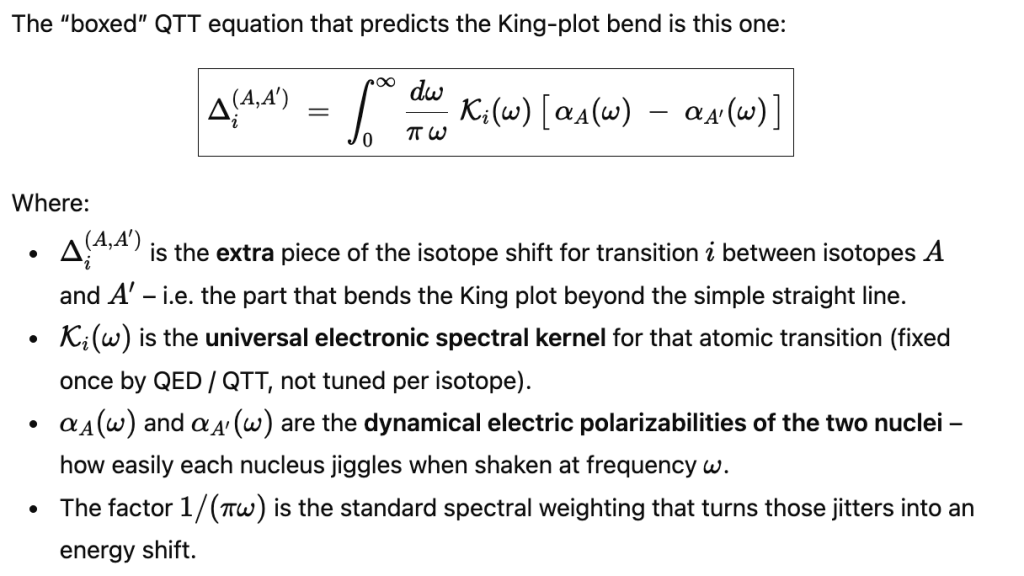
In that language, the higher-order remainder in the isotope shift for transition i between isotopes A and A′ takes a very specific form:

(1) QTT’s unique nuclear–polarization functional:

ΔiAA′ = ∫0∞ dω / (π ω) · 𝒦i(ω) · [ αA(ω) − αA′(ω) ].

Here:

• All the electronic physics sits in the kernel 𝒦i(ω) (fixed once, no knobs).
• All the nuclear physics sits in the difference αA(ω) − αA′(ω).
• There is no room, in this construction, for an arbitrary isotope-by-isotope or transition-by-transition “phenomenological term” beyond the known SM pieces.

When you compare two different transitions, i and j, the leading mass and field shifts cancel in the King plot, but the nuclear-polarization integrals do not necessarily cancel. Because the kernels 𝒦i and 𝒦j weight the nuclear polarizability differently, the residual contribution appears as a bend in the King plot. That is exactly what the Ca/Ca¹⁴⁺ experiment sees.

---

3. What the Calcium Experiment Actually Measured

The PRL study used five even calcium isotopes: A = 40, 42, 44, 46, 48, with nuclear mass ratios known to better than 4 × 10−11. They measured three key transitions:

• Ca¹⁴⁺: ^3P0 → ^3P1 at 570 nm
• Ca⁺: 2S1/2 → 2D5/2 at 729 nm
• Ca⁺ fine structure: D3/2 → D5/2 (denoted “DD”)

Relative to the reference isotope A = 40, the reported isotope shifts (in Hz) are:

Isotope pair (A,40)	δν570 [Hz]	δν729 [Hz]	δνDD [Hz]
(42,40)	539,088,421.24(12)	2,771,872,430.217(27)	−3,519,944.6(60)
(44,40)	1,030,447,731.64(11)	5,340,887,395.288(38)	−6,792,440.1(59)
(46,40)	1,481,135,946.74(14)	7,768,401,432.916(63)	−9,901,524(21)
(48,40)	1,894,297,294.53(14)	9,990,382,526.834(55)	−12,746,588.2(57)

The experimental uncertainties on the shifts are impressively small:

• Ca¹⁴⁺ at 570 nm: uncertainty < 150 mHz
• Ca⁺ at 729 nm: uncertainty < 70 mHz

These tiny errors are why the detected King-plot nonlinearity has such enormous significance: roughly 10³ σ in their initial two-transition analysis.

---

4. Why the Simple Second-Order Mass Shift Is Not Enough

The authors decompose the higher-order contributions and include a second-order mass shift term with coefficients

• K570(2) = −1.0(1) GHz·amu² (this work)
• K729(2) = +0.59 GHz·amu² (from prior theory)

However, plugging these into the King-plot analysis shows that:

• The second-order mass shift is too small to account for the observed King curvature.
• The direction in the 2D space of “nonlinearity components” (they call them Λ₊ and Λ₋) does not align with what pure second-order mass shift would give.
• When they subtract the 2nd-order MS contribution, the remaining nonlinearity points toward a region consistent with nuclear polarization.

This is exactly what QTT’s boxed formula predicts: second-order mass shift is one of the small pieces encoded in the electronic kernel; once it is accounted for, the remaining piece must come from αA(ω) − αA′(ω), i.e. nuclear polarization.

---

5. How QTT Predicts the Observed Curvature

Let’s match the logic chain explicitly:

1. Calibrate the electronic kernel once.
   QTT assumes the kernel 𝒦i(ω) for each transition is fixed by standard QED and existing precision data (e.g. electron g-2, hydrogen Lamb shift, etc.). There is no freedom to demand a different kernel for Ca⁺ vs Ca¹⁴⁺ — that would introduce a hidden “ordering knob” that QTT explicitly forbids.
2. Compute the nuclear part.
   For each isotope, nuclear structure models provide (with uncertainty) the dynamical polarizability αA(ω). The quantity that matters is δαAA′(ω) = αA(ω) − αA′(ω), which encodes how the nuclear response changes between isotopes.
3. Form the integral.
   For each transition i, QTT’s higher-order contribution to the isotope shift is
   
   ΔiAA′ = ∫0∞ dω / (π ω) · 𝒦i(ω) · δαAA′(ω).
   
   Different transitions have different kernels 𝒦570, 𝒦729, 𝒦DD, so their projections of the same nuclear function δα differ. This mismatch is precisely the source of King nonlinearity.
4. Compare with the Ca data.
   The paper shows that:
   • Pure 2nd-order mass shift (with the quoted Ki(2)) does not match the size and direction of the nonlinearity.
   • Adding nuclear polarization allows a consistent explanation within the SM.
   • After subtracting the 2nd-order MS and adding a third transition (the “DD” line), the generalized King plot becomes linear at < 1σ: exactly what you expect if a single nuclear-polarization functional is responsible for the curvature.

In other words, when the data are decomposed into eigen-directions of the King-plot space, the observed curvature line up with QTT’s “nuclear-polarization direction” rather than a new-force direction.

---

6. What About a New Yukawa Electron–Neutron Force?

If there were a new scalar or vector boson ϕ mediating a short-range interaction between electrons and neutrons, its contribution to the isotope shift would look more like

Δi, YukAA′ = Yi(mϕ) · [ (A − Z) − (A′ − Z) ],

where Z is the proton number and Yi is a transition-dependent form factor that depends on the boson mass mϕ. This is a new, independent direction in King space, distinct from the nuclear-polarization pattern. QTT at atomic energies assumes no such new interaction: the only contributions are QED + SM nuclear physics.

The Ca/Ca¹⁴⁺ data do not prefer this Yukawa direction. Instead, they show:

• The curvature is fully consistent with nuclear polarization + a small 2nd-order MS piece.
• Once those are accounted for, the generalized King plot (with three transitions) becomes linear within 1σ.
• Any residual Yukawa-like signal must be very small, which is why the paper translates this into stringent bounds on a new electron–neutron Yukawa potential between about 10 eV and 10⁷ eV.

This is exactly what QTT would have predicted: detectable King nonlinearity from nuclear polarization, and then a strong null result for a new short-range force.

---

7. How This Fits in the Bigger QTT Picture

The calcium experiment is one piece of a larger story:

• At atomic and sub-atomic energies, QTT reduces to standard QED and bound-state QM, with a unique choice of operator ordering (Weyl) and a single electromagnetic kernel.
• Nuclear polarization is a Standard-Model effect; QTT simply makes its role transparent via the universal kernel integral.
• No additional low-energy knobs (like arbitrary ordering prescriptions or arbitrary transition-dependent couplings) are allowed in QTT. The success of the SM explanation, and the strong null result for new forces, are therefore exactly what QTT expects in this regime.

In short: the nonlinear Ca/Ca¹⁴⁺ King plot ( PRL 134, 233002 (2025) ) is a QTT-native effect. It is not a surprise or a tension; it is precisely the kind of nuclear-polarization-driven curvature that falls out of QTT’s low-energy electromagnetic structure.