The Smallest Receipt: The Largest Fact That Both Quantum Mechanics and General Relativity Ignored
What Artian's Ruler is, why it is not simply the Planck length, and how QTT meters it without Newton's constant
This essay explains a QTT-native source construction and a target-visible, zero-fit, non-gravitational metrology audit. The conventional Planck length and the measurements of 


Most people meet the Planck length as a number:

It is so small that ordinary comparisons become ridiculous. A proton is enormous next to it. An atom is enormous next to a proton. A human hair, compared with this scale, might as well be an astronomical object.
That usually ends the explanation. The Planck length is introduced as the place where quantum mechanics and gravity are expected to stop ignoring each other. It is built from three constants,

and then treated as nature's smallest meaningful ruler.
The equation is correct. The interpretation is less complete than it first appears. It tells us how to assemble a length from ħ,
That last problem bothered me. If I use

I have not derived
Quantum Traction Theory takes the order seriously. The source ruler must exist before gravity reads it. Gravity can be a downstream response to the ruler. It cannot be smuggled upstream to manufacture the ruler and then be announced as its consequence.
QTT therefore uses a different name:

The different symbol is not branding. It protects a different constructor, a different ontology, and a different scientific burden. The conventional Planck length is a gravitational combination. Artian's Ruler is the proposed stride of one completed physical address in Artian geometry. Its source definition comes first. Its numerical value in metres comes through a declared measurement door. Its comparison with the conventional Planck ruler comes last.
This Field Note is the long version of that statement. I will explain what 
There is no shortcut through this one. The details are the defense.
Section 1Two rulers that currently land in almost the same place
Let us put the numbers on the table first.
The current weak-sector QTT construction gives

before uncertainty rounding, or
%5Ctimes10%5E%7B-35%7D%5C%20%5Cmathrm%20m.%0A%7D&bg=101b30&fg=f5f0e5&s=1&c=20201002)
The conventional CODATA-2022 gravitational ruler gives

Their central-value ratio is

That is a difference of about 106 parts per billion.
The Artian value is slightly larger. The difference matters as an audit receipt because the two numbers were constructed through different routes. It does not establish that nature contains two experimentally distinct microscopic lengths. The uncertainty of the conventional ruler is inherited from
CODATA's relative uncertainty for
%3D22.474%5C%20%5Cmathrm%7Bppm%7D.&bg=101b30&fg=f5f0e5&s=1&c=20201002)
Because the conventional Planck length depends on 
%3D11.237%5C%20%5Cmathrm%7Bppm%7D.&bg=101b30&fg=f5f0e5&s=1&c=20201002)
The weak-sector Artian construction has a metrological uncertainty of
%3D0.2572%5C%20%5Cmathrm%7Bppm%7D%2C&bg=101b30&fg=f5f0e5&s=1&c=20201002)
conditional on the QTT source kernel. The conventional comparator is therefore about 44 times less precise at the metrology layer.
The central difference of 


So the correct reading is this:
The two constructions currently agree extremely well. They are not experimentally resolved as different. The separate name is justified by source order and physical meaning, not by claiming that the
If future measurements of
Section 2What a ruler means in Artian geometry
The word ruler can be misleading.
In QTT, a physical address is earned when an event closes. The address is a receipt of a completed physical act. Three ledgers close together:

Each equation has a different job.
The first is modular closure. The event must complete one full bundle:

An incomplete turn may be a source process on its way to closure. It is not yet a completed address.
The second is the action ledger:

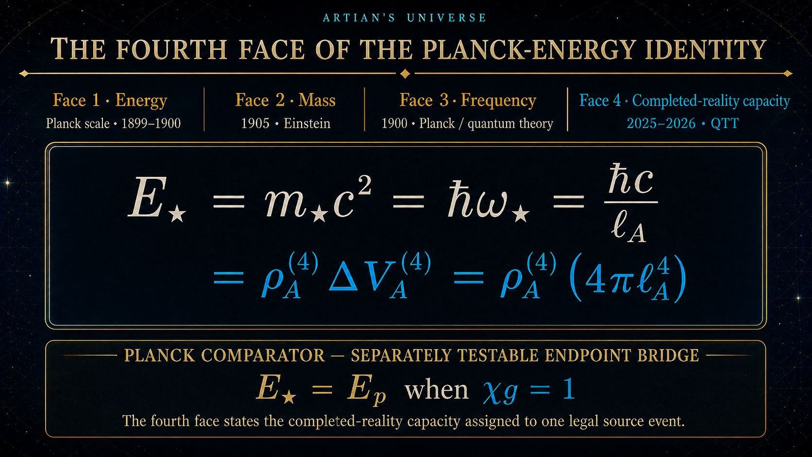
One completed event spends one quantum of action over one Artian tick. The endpoint event carries the maximum legal energy 

The source carrier speed is

The third relation gives one completed event finite four-volume support:

This is where the geometry differs from a naked cube. The 
The important word is legal. QTT does not claim that a mathematician is forbidden to write 

Suppose we try to make the completed tick shorter while keeping one full action quantum:

If

then

That exceeds the endpoint capacity. The proposed event asks one address to carry more than the maximum funded energy. It is not another smaller address. It is an illegal over-capacity request.
The argument can be written as a compact conditional theorem:

and therefore

That is why QTT calls
Section 3The internal geometry before metres exist
QTT separates the form of the ruler from its numerical calibration.
Before anyone asks how many metres

Twenty-four such volume shares close one rotational space quantum:
%0A%3D4%5Cpi%5Cell_A%5E3.%0A%7D&bg=101b30&fg=f5f0e5&s=1&c=20201002)
The number 

One Artian tick contributes another factor of the ruler, giving the completed four-volume:

The two-sided surface tile is built from

and the 32-face closure count:

These relations close exactly:
%5E2%0A%3D64%5Cpi%5E2%5Cell_A%5E4%0A%3D16%5Cpi%5Cleft(4%5Cpi%5Cell_A%5E4%5Cright)%0A%3D16%5Cpi%5CDelta%20V_4.&bg=101b30&fg=f5f0e5&s=1&c=20201002)
So

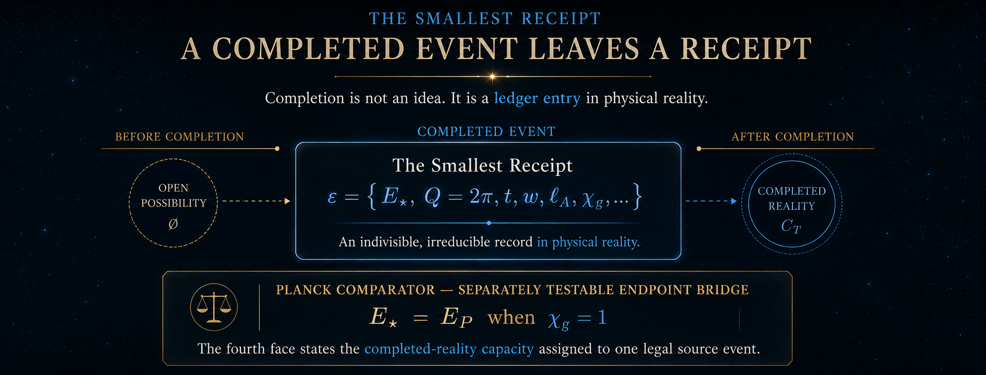
2π modular bundle, one Eℰt̃A = ħ action-throughput closure, and one ΔV4,ℰ = 4πℓA4 support. χg belongs to the separate endpoint camera: χg = 1 is the preregistered EFA-G1 hypothesis, not a consequence of A2+A5-X+A6+A7. One completed event is one irreducible ledger increment even when its later physical record has distributed support.This internal geometry says what kind of object
This distinction is easy to miss. Integers, angles, topology, and dimensionless closure rules cannot produce a number carrying metres all by themselves. Any theory claiming otherwise has hidden a ruler somewhere. QTT's current strongest executed route declares its ruler openly: it uses the measured weak constant
That makes the result non-
The source-only SI programme has a separate caesium bridge. Its exact factorization is closed, but the latest frozen universal alkali identity word failed transfer to rubidium and potassium. The required nuclear magnetic and electronic-contact source operators remain open. That failure is useful. It prevents one accurate caesium landing from being promoted into a source law it has not earned.
Section 4Why the conventional Planck ruler and Artian's Ruler begin in opposite directions
The conventional construction starts with gravity:

QTT starts with a completed source endpoint:

The algebraic connection is clear:

The ontological order is different. QTT treats 
This makes the metrology question sharp. Can
The current paper answers conditionally: yes, through the weak scalar and photon-edge route.
Section 5The whole constructor in one line
The final non-
%7D%0A%3D2%5E%7B3%2F4%7D%5Chbar%20c%5C%2C%0Aq_H%5Cmathcal%20R_H%5E%7B%5Crm%20EW%7D%5Csqrt%7BG_F%7D.%0A%7D&bg=101b30&fg=f5f0e5&s=1&c=20201002)
This equation is compact enough to look suspicious. A reader sees 


The defense is to open every box.
The constructor contains four kinds of ingredient:
| Ingredient | Expression | Role |
|---|---|---|
| Exact SI bridge | ħ and | Converts inverse energy into length |
| Measured dimensional anchor | | Meters the weak scale through muon decay |
| Measured dimensionless edge input | &bg=0b1424&fg=f5f0e5&s=0&c=20201002) | Supplies a very small electromagnetic readout correction |
| QTT source objects |  , , , , | Specify the weak-to-endpoint map |
The forbidden constructor list is equally important:

The gravitational ruler is opened only after
Section 6The measured weak door:
The Fermi constant is extracted from the positive muon lifetime. In the low-energy weak description,
%2C&bg=101b30&fg=f5f0e5&s=1&c=20201002)
where 

The primary input used in the metrology paper is
%5Ctimes10%5E%7B-5%7D%5C%20%5Cmathrm%7BGeV%7D%5E%7B-2%7D.%0A%7D&bg=101b30&fg=f5f0e5&s=1&c=20201002)
This is measured physics, but it is not theory-free. The conversion from muon lifetime to
The operational Fermi ruler is
%5E%7B-1%2F2%7D%0A%3D246.2196508%5C%20%5Cmathrm%7BGeV%7D.%0A%7D&bg=101b30&fg=f5f0e5&s=1&c=20201002)
The phrase operational Fermi ruler is deliberate. Beyond tree level, one should not silently identify it with every gauge- and scheme-dependent definition of a renormalized Higgs vacuum expectation value. This calculation spends the low-energy ruler determined by muon decay. It does not fit a Higgs potential to obtain it.
There is also a basic dimensional reason
![\displaystyle [G_F]=E^{-2},
\qquad
[\sqrt{G_F}]=E^{-1}.](https://s0.wp.com/latex.php?latex=%5Cdisplaystyle%20%5BG_F%5D%3DE%5E%7B-2%7D%2C%0A%5Cqquad%0A%5B%5Csqrt%7BG_F%7D%5D%3DE%5E%7B-1%7D.&bg=101b30&fg=f5f0e5&s=1&c=20201002)
Since
![\displaystyle [\hbar c]=EL,](https://s0.wp.com/latex.php?latex=%5Cdisplaystyle%20%5B%5Chbar%20c%5D%3DEL%2C&bg=101b30&fg=f5f0e5&s=1&c=20201002)
the combination

has units of length.
That dimensional fact is not the discovery. Anyone can multiply a measured inverse-energy scale by a dimensionless number. The scientific content is whether QTT fixes the dimensionless number independently and restricts the allowed alternatives.
Without the QTT attenuation,

which is nowhere near the Planck scale. The constructor must supply a further factor of about 
Section 7The completed projected bundle: why ρ is there
QTT uses one real modular dial. A completed turn carries

The laboratory does not read the source dial face-on. A1 assigns the two-clock projection angle

The projected completed loop is therefore
.%0A%7D&bg=101b30&fg=f5f0e5&s=1&c=20201002)
Numerically,
%0A%3D0.923879532511%5Cldots&bg=101b30&fg=f5f0e5&s=1&c=20201002)
and

Why 
Why 
Why multiply them? Because ρ is the laboratory projection of the completed bundle loop, not a new free constant.
The reuse helps only under no-retune discipline. QTT cannot change ρ to save the ruler without moving every other sector that uses the same object. Those rows are correlated, so they cannot be multiplied into fake independent significance. They do make the constructor more expensive to repair after a failure.
Section 8The scalar-lock graph: why there are three vertices
The weak scale is treated as a visible scalar share of the completed endpoint bundle. The route from the source bundle to the laboratory has three typed stages:


Among these three vertices there are three possible forward edges. Each edge can be present or absent, producing

edge subsets.
The paper enumerates all eight. The declared admissibility rules require source-to-readout connection, mandatory locking, order, minimality, and no bypass. Only the serial route survives.
This is a real defense against local formula shopping. It is still scoped. The result is unique inside the printed three-vertex grammar. It does not prove that no other effective theory or arbitrary function could imitate the final number.
The next paper should make this boundary even harder by deriving the admissibility class itself directly from the axioms. I return to that later.
Section 9Why the attenuation is exponential
The two legal gates carry actions. A serial traversal pays both. In QTT's finite-address kinetic ledger, a gate with action 

Serial gates multiply:
%7D.&bg=101b30&fg=f5f0e5&s=1&c=20201002)
The real completed dial has two allowed orientations. That gives the leading multiplicity 

The exponential is therefore tied to additive gate action along the unique serial chain. It is not introduced merely because exponentials are good at producing very small numbers.
That source rule remains a QTT theorem, not a Standard Model consequence. A critic is entitled to challenge it. The paper's job is to make the challenged premise visible.
Section 10Why the dominant action is exactly 
The first gate joins visible and hidden completed modular coordinates. Each coordinate closes over one full
![\displaystyle \phi_{\rm vis}\in[0,2\pi],
\qquad
\phi_{\rm hid}\in[0,2\pi].](https://s0.wp.com/latex.php?latex=%5Cdisplaystyle%20%5Cphi_%7B%5Crm%20vis%7D%5Cin%5B0%2C2%5Cpi%5D%2C%0A%5Cqquad%0A%5Cphi_%7B%5Crm%20hid%7D%5Cin%5B0%2C2%5Cpi%5D.&bg=101b30&fg=f5f0e5&s=1&c=20201002)
The product-face action is

Therefore,

The number is an area in modular-coordinate space. It is not one circumference counted twice for decoration. Two independently completed coordinates form a product face, and the face area is 
This term does almost all the hierarchy work:

Once the orientation factor 
The physical burden is clear. If the visible-hidden scalar lock does not own this completed product face, the dominant attenuation fails. The impressive decimal landing cannot rescue the ontology after the fact.
Section 11Why the radial action is exactly &bg=0b1424&fg=f5f0e5&s=0&c=20201002)
The second action is smaller, but it is structurally important. Start with the projected radial-square kernel

The neutral dyadic gate is

It acts on both sides of the quadratic kernel:

The factor 
%5E2%3D%5Cfrac14.&bg=101b30&fg=f5f0e5&s=1&c=20201002)
The tangential direction has already been removed. The rank-one radial projector 

Therefore,
%0A%3D%5Cfrac12%5Cleft(%5Cfrac%7B1%7D%7B4%5Crho%5E2%7D%5Cright)%0A%3D%5Cboxed%7B%5Cfrac%7B1%7D%7B8%5Crho%5E2%7D%7D.&bg=101b30&fg=f5f0e5&s=1&c=20201002)
The denominator eight has a ledger:

The 
Numerically,

This action is tiny next to
Section 12Why the prefactor is
The prefactor in
%7D&bg=101b30&fg=f5f0e5&s=1&c=20201002)
counts the two orientations of a real closed dial. A completed circle can be traversed with either orientation. The multiplicity is discrete. It is not a continuous normalization adjusted to the weak scale.
This factor is load-bearing. Removing it would cut
That sensitivity is not a weakness if the orientation count is independently forced. It is exactly what makes the statement falsifiable. If the source geometry permits one orientation, four orientations, or an unconstrained multiplicity, the ruler theorem loses its rigidity.
With all pieces assembled,
![\displaystyle \boxed{
q_H
=2\exp\left[-4\pi^2-\frac{1}{8\rho^2}\right]
=1.42613305080570\times10^{-17}.
}](https://s0.wp.com/latex.php?latex=%5Cdisplaystyle%20%5Cboxed%7B%0Aq_H%0A%3D2%5Cexp%5Cleft%5B-4%5Cpi%5E2-%5Cfrac%7B1%7D%7B8%5Crho%5E2%7D%5Cright%5D%0A%3D1.42613305080570%5Ctimes10%5E%7B-17%7D.%0A%7D&bg=101b30&fg=f5f0e5&s=1&c=20201002)
This number is the proposed visible Higgs/scalar subcharge of one completed endpoint bundle.
Section 13The electroweak edge: why α and why the square root contains six
The raw scalar lock does not quite equal the laboratory Fermi ruler. QTT attaches a small finite electroweak readout gate:
![\displaystyle \boxed{
\mathcal R_H^{\rm EW}
=\exp\left[
-\frac{\alpha(0)}{8\rho^2}
\sqrt{6+\rho^{-2}}
\right].
}](https://s0.wp.com/latex.php?latex=%5Cdisplaystyle%20%5Cboxed%7B%0A%5Cmathcal%20R_H%5E%7B%5Crm%20EW%7D%0A%3D%5Cexp%5Cleft%5B%0A-%5Cfrac%7B%5Calpha(0)%7D%7B8%5Crho%5E2%7D%0A%5Csqrt%7B6%2B%5Crho%5E%7B-2%7D%7D%0A%5Cright%5D.%0A%7D&bg=101b30&fg=f5f0e5&s=1&c=20201002)
This factor is close to one:

It does not create the 
The measured coupling is the Thomson-limit fine-structure constant,
%5E%7B-1%7D%3D137.035999177.&bg=101b30&fg=f5f0e5&s=1&c=20201002)
The paper uses measured α deliberately. This keeps the metrology question narrow. The wider QTT corpus has a photon-edge construction for α, but silently substituting that value would change the epistemic class of this calculation. A source-α branch should be frozen and reported separately.
Now the number six.
The finite electroweak readout complex contains three broken electroweak directions. Each has two real 

The readout vector is

so its squared norm is

The six unit entries represent the three broken directions and their real quadratures. The final 
The neutral boundary pullback is

The canonical first readout moment becomes

The single-kernel electromagnetic window contributes one half of α:

Finally,

Numerically,


and

Every number now has a named origin. Whether those origins describe nature is the scientific question. Their presence is no longer unexplained arithmetic.
Section 14The scalar lock and its two square roots of two
The QTT weak-to-endpoint relation is

The first √2 belongs to the QTT dyadic scalar-lock boundary. It converts the one-root scalar share into the laboratory Fermi ruler.
The standard weak definition also contains √2:
%5E%7B-1%2F2%7D.&bg=101b30&fg=f5f0e5&s=1&c=20201002)
These two appearances produce the
Invert the QTT lock:

Insert the measured weak ruler:
%5E%7B-1%2F2%7D%7D%0A%7B%5Csqrt2%5C%2Cq_H%5Cmathcal%20R_H%5E%7B%5Crm%20EW%7D%7D.&bg=101b30&fg=f5f0e5&s=1&c=20201002)
The result is

This endpoint is a capacity scale. It is not a predicted particle resonance at 
Now convert the endpoint into Artian's Ruler:

Substitution gives
%5E%7B1%2F2%7D.&bg=101b30&fg=f5f0e5&s=1&c=20201002)
The powers are
%5E%7B1%2F2%7D%3D2%5E%7B1%2F4%7D.&bg=101b30&fg=f5f0e5&s=1&c=20201002)
Therefore,

and

The apparently unusual
Section 15Walking through the arithmetic without hiding the scale
Use the exact SI conversion

The weak anchor contributes

Their product is roughly

The remaining dimensionless factor is

Multiplying gives
%0A(2.398%5Ctimes10%5E%7B-17%7D)%0A%5Capprox1.616%5Ctimes10%5E%7B-35%7D%5C%20%5Cmathrm%20m.&bg=101b30&fg=f5f0e5&s=1&c=20201002)
The 80-digit certificate evaluates two independent algebraic paths:
%7D%0A%3D2%5E%7B3%2F4%7D%5Chbar%20c%20q_H%5Cmathcal%20R_H%5E%7B%5Crm%20EW%7D%5Csqrt%7BG_F%7D%2C&bg=101b30&fg=f5f0e5&s=1&c=20201002)
and
%7D%0A%3D%5Cfrac%7B%5Chbar%20c%7D%7BE_%5Cstar%7D%2C%0A%5Cqquad%0AE_%5Cstar%0A%3D%5Cfrac%7B(%5Csqrt2G_F)%5E%7B-1%2F2%7D%7D%0A%7B%5Csqrt2q_H%5Cmathcal%20R_H%5E%7B%5Crm%20EW%7D%7D.&bg=101b30&fg=f5f0e5&s=1&c=20201002)
They agree to better than 
Section 16The no-smuggling derivative
Leaving
The logarithmic sensitivities are


and

The first equation says a one-part-per-million shift in
The second says the current α uncertainty contributes almost nothing to the ruler uncertainty because the electroweak edge is very small.
The third is the constructor firewall. Newton's constant has exactly zero influence on the Artian result.
This is stronger than a visual inspection. It gives the claim an executable mathematical form:

If a later version introduces 


Section 17Why the slightly different number makes the separate name appropriate
There are two reasons for the name Artian's Ruler. Only one of them is numerical.
The primary reason is constructor identity.

inside a completed-address geometry. Its current numerical value is obtained through a weak-sector door. The conventional Planck length is defined by

Two quantities can be numerically equal and still deserve different symbols when their definitions, dependencies, or operational meanings differ. Physics does this constantly. Equality becomes a theorem or empirical identification, not a typographical assumption.
The secondary reason is that the current central values are not exactly equal:

That difference demonstrates that the weak-sector constructor is not algebraically forced to copy the current CODATA
This is the accurate language:
are distinct constructor objects whose current central values are extremely close. Their physical identification remains a testable QTT bridge.
If future
The endpoint-gain ledger makes that future possibility precise. QTT now writes

The core axioms do not force 

then

The current tiny central offset could therefore be written as a central-value estimate of an endpoint gain slightly below one. Present
Section 18Three reasons the comparison is genuinely good despite poor
The weak precision of
Reason 1: the constructor is independent of the comparator
The Artian route uses

The agreement is therefore not the inevitable result of substituting
Reason 2: the landing is near the comparator's centre, not merely somewhere inside its broad uncertainty band
The
The local ablation scan also matters:
| Frozen local branch | Length residual |
|---|---|
| Modular area only |  ppm ppm |
| Modular area plus electromagnetic edge |  ppm ppm |
| Modular area plus radial action |  ppm ppm |
| Full printed constructor |  ppm ppm |
Only the full branch lies within one part per million among the declared 16 local alternatives. This does not calculate a universal chance probability. It shows that the nearby typed operations are not interchangeable decorations.
Reason 3: the imprecision of creates a clean prospective direction
The Artian metrology layer is much narrower than the current gravitational comparator. Conditional on the source theorem,
while
The weak route therefore prints a much sharper place for future gravitational metrology to test. QTT cannot claim victory now, but it can freeze the target. If independent future

without any change to
Poor
Section 19Why this is not defended by the decimal alone
A number this close to a known target should trigger suspicion. That is healthy.
The defense cannot be “look how many digits agree.” Formula searches can produce impressive coincidences, especially when the target is already visible. The defense has to come from the constructor ledger:
- The source object is named before comparison.
- Every allowed operation has a physical role.
- The finite graph alternatives are enumerated.
- Nearby action branches are published, including failures.
- Measured anchors are declared instead of being called derived constants.
- Reused objects cannot be retuned sector by sector.
- The target-visible chronology is admitted.
- Structural theory uncertainty is marked not identified, not zero.
- Future no-retune falsifiers are printed.
The Constructor Alphabet paper adds another layer. It asks how often a frozen symbolic language can imitate a target after accounting for allowed leaves, operators, complexity, dependencies, and chronology. It does not assign a fake universal probability to all equations humans might imagine. It classifies the claim correctly: scalar corridors, exact identities, finite enumerations, and structural laws require different null models.
For this ruler, the correct statement is:

The calculation is a Class-A Keystone result. It uses one declared measured dimensional anchor. Its algebra, local graph uniqueness, unit closure, and no-smuggling firewall are closed inside the printed construction. Its physical source hypotheses and structural covariance remain under test.
Section 20What would falsify or weaken the Artian's Ruler route
The route should be considered damaged if any of the following occurs:
- The scalar-lock graph class permits a second inequivalent admissible route under the same rules.
- The product-face action
- The radial action
- The orientation multiplicity is not exactly two.
- The electroweak readout complex does not contain the stated six broken
- A future branch is selected because it improves the known Planck residual.
- Improved
- QTT changes ρ,
- The eventual structural covariance is large enough that the numerical landing carries little evidential weight.
A source-only SI failure does not automatically falsify the weak-anchored route. It would show that QTT has not yet derived the metre from source law alone. Conversely, success of the weak route does not close the caesium nuclear packet. The status layers remain separate.
Section 21What the result does not claim
The Artian's Ruler paper does not establish all of QTT from one number.
It does not claim:
- A blind prediction of the Planck length.
- A Planck-scale particle accessible to an accelerator.
- A perturbative ultraviolet completion of the Standard Model.
- A derivation of α within the headline metrology branch.
- A source-only derivation of the SI metre.
- Zero structural theory uncertainty.
- A global look-elsewhere probability.
- Six statistically independent confirmations of one ruler.
- Experimental proof that
- Proof that the universal gravitational endpoint gain is exactly one.
It does claim something narrower and worth checking:
Given the printed QTT scalar-lock source construction, the measured weak scale reconstructs a finite capacity endpoint and a microscopic length without using Newton's constant. The result is dimensionally closed, locally unique inside the declared graph grammar, zero-fit with respect to the Planck target, and centrally consistent with the conventional gravitational ruler.
That statement is strong enough. There is no need to inflate it.
Section 22What I would improve in the next Artian's Ruler paper
Writing the whole route in one place exposes several useful next steps.
Section 22.1Prove the minimum-ruler theorem explicitly
The source logic is already present, but the paper would benefit from a named theorem:

The theorem should list exactly which axiom supplies each premise and distinguish an incomplete coordinate subdivision from a legal completed physical address.
Section 22.2Derive the graph grammar, not only the winning graph
Enumerating eight graphs is useful. A sharper result would prove why
Section 22.3Add a typed dependency diagram for every numeral
The paper should include one machine-readable graph connecting

to their source roles, first publication dates, allowed operations, downstream equations, and falsifiers. This would make the anti-numerology defense inspectable without reading the entire corpus.
Section 22.4Freeze two α branches
The current metrology branch uses measured

the numerical difference is tiny. The epistemic difference is large: one branch is weak-anchored plus measured edge input; the other asks whether the source photon-edge theorem carries the readout by itself.
Section 22.5Publish a structural covariance instead of leaving it NI
The metrological uncertainty is already propagated. The source uncertainty is marked

The next version should define a principled uncertainty or model-credence ledger over the finite graph class, action ownership, projection rule, and edge-map alternatives. It should not invent a Gaussian error bar for axioms. A discrete robustness or theorem-dependency analysis may be more honest.
Section 22.6Turn the offset into a preregistered endpoint-gain test
The relation

connects a future resolved ruler difference to the universal endpoint gain. The paper should freeze how post-publication 
Section 22.7Add an independent non- ruler door
The strongest improvement would be a second dimensional route that uses neither
Section 22.8Integrate the failed K2 transfer honestly
The source-only SI discussion should include the v8 caesium result: exact K2 factorization remains; the frozen universal alkali identity word failed badly on rubidium and potassium; the nuclear magnetic and electronic contact operators remain to be built. This is not an embarrassment to remove. It shows that the corpus can distinguish an accurate landing from a transferable source theorem.
Section 22.9Normalize the public endpoint digits
The current v8 numerical certificate gives

rounded in the paper to

Some public summary text carries a slightly different final digit sequence. The Zenodo description, DOI Map, gravity page, certificate, and future blog card should be normalized to the machine certificate.
Section 22.10State the naming theorem
The paper should explicitly say:

The notation 
Section 23A high-school version of the entire argument
Imagine a factory that sells one tiny kind of sealed box.
Each legal box must satisfy three rules. Its locking dial has to make one complete turn. It must receive exactly one token of action during one factory tick. It must occupy one complete unit of supported space and time.
There is also a maximum amount of energy the factory can fund in one box. Call it
Light travels a distance

during that tick. That is Artian's Ruler.
Trying to make a smaller legal box while keeping the full action token would demand more than
Now imagine that we cannot see the factory's full capacity directly. We can see one weak output line. QTT says the weak output is a tiny, precisely structured share of the full endpoint. The share is 
Muon decay tells us the size of the weak output. Divide by the frozen share and we infer the full factory capacity 
Only then do we open the separate gravity invoice and ask whether its Planck ruler lands in the same place.
It does, to within 
That is the result.
Section 24The deeper ontological point
The Planck length is usually introduced as a scale where our equations become uncomfortable. Artian's Ruler is introduced as the scale at which one physical address becomes complete.
That difference changes the question.
Instead of asking, “How small can a coordinate become?”, QTT asks, “What is the smallest completed event that can carry one legal action token without exceeding one finite capacity endpoint?”
Instead of asking gravity to define the ruler, QTT asks several sectors to read the same source ruler through different doors.
Instead of assuming that an infinitesimal point can support unlimited physical bookkeeping, QTT requires a finite address receipt:

The ruler, tick, endpoint, surface tile, and gravity coefficient then form one connected ledger:

These are not four independent numerical successes. They share one source degree of freedom. Their economy is also their evidential limit. A single independent non-gravitational measurement of the ruler can propagate through the whole network. It cannot be counted as four separate confirmations.
The value of the framework lies in making that dependency visible.
Section 25The strongest honest claim
Here is the statement I am prepared to defend:
QTT assigns its smallest physical ruler to the stride of one completed finite-capacity address. The ruler is conjugate to a maximum one-event capacity through. A declared weak-sector scalar-lock constructor uses the measured Fermi constant and a small electromagnetic edge input to meter this ruler without Newton's constant. The resulting value,
m, is centrally
That is already a substantial result. It gives the Planck-scale length a source object, a measurement route, an audit trail, and a clear place to fail.
The next step is not another decimal. It is another independent door.
Related papers and reader anchors
- Quantum Traction Theory: Main Book, v10.01
Concept DOI: 10.5281/zenodo.17527179
Main source anchors: completed addresses and the noncircular ruler, pp. 52-61; projected dial, pp. 158-160; endurance/gravity readout, pp. 199-204; scalar-lock and weak hierarchy, pp. 971-985. - Planck-length metrology without Newton's constant
Concept DOI: 10.5281/zenodo.21190193
The complete weak-sector construction, graph enumeration, local branch scan, uncertainty propagation, and - Artian Capacity Endpoint Without G
Concept DOI: 10.5281/zenodo.21182051
Separates non- - Newton's Constant Is Not Primitive in QTT
Concept DOI: 10.5281/zenodo.20057430
Carries the endurance identity (G_A=\ell_A^2c^3/\hbar) and the correlated cross-sector endpoint ledger. - The Artian Keystone Audit
Concept DOI: 10.5281/zenodo.21141060
Classifies unconditional, anchored, keystone-dependent, and structural rows and audits the provenance of ρ, - The Constructor Alphabet Under a Dependency-Conditioned Null Model
Concept DOI: 10.5281/zenodo.21182091
The corpus-wide anti-numerology and trials-exposure audit. - The Photon-Edge Gate
Concept DOI: 10.5281/zenodo.20628735
The five-rail source construction behind the QTT fine-structure branch. - Artian Source-Only SI Endpoint Bridge Theorem
Concept DOI: 10.5281/zenodo.20936013
Separates the exact SI readout bridge from the still-open caesium source packet. - Artian Source-Only SI Closure: the K2 Caesium Hyperfine Source Packet Theorem
Concept DOI: 10.5281/zenodo.21249436
Preserves the exact K2 factorization, reports the failed universal alkali transfer, and localizes the missing nuclear and electronic operators. - Three Readouts, One Surface Tile
Concept DOI: 10.5281/zenodo.21249112
Connects the Artian surface tile to Newton, Planck, and the Bekenstein count while exposing their rank-one dependence. - No-Go Theorem and Conditional Uniqueness for the Universal Endpoint Gain
Concept DOI: 10.5281/zenodo.21955408
Proves that the core source axioms do not by themselves force - Runnable verification surface
Concept DOI: 10.5281/zenodo.21138431
Website anchors:
- Artian's Ruler in the QTT Lexicon
- Artian micro-ruler
- Non-gravitational Artian's Ruler corridor
- Source-only SI endpoint bridge
- Keystone class
- Gravity reference surface
- Corpus Tree
- Derivation Atlas
- Observatory
Standard-physics sources used by the metrology route
- V. Tishchenko et al., Detailed report of the MuLan measurement of the positive muon lifetime and determination of the Fermi constant, arXiv:1211.0960.
- P. J. Mohr, E. Tiesinga, D. B. Newell and B. N. Taylor, *CODATA recommended values of the fundamental physical constants: 2022*, Reviews of Modern Physics 97, 025002 (2025).
- C. Rothleitner and S. Schlamminger, *Measurements of the Newtonian constant of gravitation, G*, Review of Scientific Instruments 88, 111101 (2017).
Continue through the ruler corridor
Where Artian's Ruler lives in the main book
QTT Main Book v10.01 · stable concept DOI 10.5281/zenodo.17527179.
- pp. 52-61: completed addresses and the non-circular ruler.
- pp. 158-160: projected dial and the π/8 access angle.
- pp. 199-204: endurance and the downstream gravity readout.
- pp. 971-985: scalar lock, weak hierarchy, and the endpoint corridor.
Blog Map and corpus anchors
Use the Blog Map for the Field Note series, the Corpus Tree for the citable paper family, and the Lexicon for the canonical term.