How Quantum Traction Theory Shows Slowing Cosmic Acceleration and Explains the Hubble Tension

Today, I was watching https://www.youtube.com/watch?v=iUgqNu9cOEA related to #Astrum . I though to prepare a blog to solve it for them. Creation law and blops powering up our universe :).

So like other blogs, our reference: https://doi.org/10.5281/zenodo.17594186

Standard cosmology says the universe is expanding faster and faster, driven by a mysterious “dark energy” with almost constant density. At the same time, measurements of today’s Hubble constant \(H_0\) disagree depending on how you measure it: the CMB prefers a lower value, while local distance ladders prefer a higher one. This is the Hubble tension.

Quantum Traction Theory (QTT) offers a different perspective:

  • the universe in its absolute clock is on a coasting expansion,
  • apparent acceleration comes from a creation–driven time drift,
  • and the Hubble tension is a manifestation of environment‑dependent drift, not conflicting values of a fundamental constant.

Crucially, the same creation law that slows down cosmic acceleration also naturally spreads measured \(H_0\) values between different probes.


1. Two clocks and coasting expansion in QTT

QTT distinguishes between:

  • an absolute background clock \(T\) (ABC time), and
  • local laboratory time \(t_{\rm lab}\), the time we actually measure.

Axiom A1 gives:

\[ d\tau = N(x^\mu,v)\,dT, \]

where \(N(x^\mu,v)\) is the usual gravitational/kinematic lapse; in cosmology we can take \(N\simeq 1\) at the background level. The second key choice is the coasting gauge:

\[ a(T) \propto T, \qquad H_\tau(T) := \frac{1}{a}\frac{da}{dT} = \frac{1}{T}. \]

So in ABC time the expansion is exactly coasting:

  • no acceleration: \(d^2 a/dT^2 = 0\),
  • Hubble in ABC time: \(H_\tau(T) = 1/T\).

The observational drama enters when we ask:

What is the Hubble parameter when measured in lab time, not in ABC time?


2. Time Tilt, Time Drift, and the mapping t ↔ T

In QTT, lab time is a tilted, drifting axis inside a 2D time plane spanned by \(T\) and a hidden reality direction \(w\). The local relation between lab time and ABC time is:

\[ dt_{\rm lab}(x,v;a) = I_{\rm clk}\,F_{\rm drift}^{\rm (time)}(a,x)\,N(x^\mu,v)\,dT. \]

  • Tilt: a universal factor \(I_{\rm clk} = \cos(\pi/8)\), fixed by QTT’s discrete time‑plane symmetry.
  • Drift (time version): \(F_{\rm drift}^{\rm (time)}(a,x)\), a slow, environment‑dependent factor coming from the Law of Creation.
  • Dilation: \(N(x^\mu,v)\), the usual GR/SR lapse (≈1 for background cosmology).

For cosmological backgrounds we drop \(x,v\) and set \(N\simeq 1\), so

\[ dt_{\rm lab}(a) = I_{\rm clk}\,F_{\rm drift}^{\rm (time)}(a)\,dT. \]

For rates like Hubble, it is convenient to invert this and package Drift as a factor multiplying H rather than time intervals. Define the rate–drift factor:

\[ F_{\rm drift}^{\rm (rate)}(a) := \frac{I_{\rm clk}}{F_{\rm drift}^{\rm (time)}(a)}. \]

Then

\[ \frac{dT}{dt_{\rm lab}} = \frac{1}{I_{\rm clk}\,F_{\rm drift}^{\rm (time)}} = \frac{F_{\rm drift}^{\rm (rate)}}{I_{\rm clk}^2}. \]

For our purposes we only need the combination that multiplies \(H_\tau\), so we simply write:

\[ H_{\rm lab}(a,{\rm env}) = \frac{1}{a}\frac{da}{dt_{\rm lab}} = \frac{H_\tau(T)}{I_{\rm clk}}\,F_{\rm drift}^{\rm (rate)}(a,{\rm env}), \tag{1} \label{eq:Hlab-def} \]

where “env” labels the astrophysical environment behind the probe (CMB, TRGB, Cepheids, etc.). The key point:

  • Coasting in \(T\): \(H_\tau(T) = 1/T\) is universal.
  • Differences in measured \(H_0\) come entirely from \(F_{\rm drift}^{\rm (rate)}\), which depends on creation and environment.

3. Creation law and the drift integral

Where does \(F_{\rm drift}\) come from? QTT ties it directly to the Law of Creation via a time‑plane angle \(\theta(a)\). The lab axis \(u_t\) sits at an angle \(\theta(a)\) relative to the absolute axis \(u_\tau\). We write:

\[ \theta(a) = \theta_\ast + \delta(a), \qquad \theta_\ast = \frac{\pi}{8}, \]

with \(\theta_\ast\) the universal tilt and \(\delta(a)\) a slow, creation‑driven drift. The macroscopic QTT drift law is:

\[ \boxed{ \delta(a) \simeq \frac{1}{3} \int_0^{a} \Bigl[ \Omega_m(\tilde a) + \tau(\tilde a)\,\Omega_{\rm cre}(\tilde a) \Bigr]\, d\ln\tilde a, } \tag{2} \label{eq:delta-drift} \]

with

  • \(\Omega_m(a)\) = matter fraction,
  • \(\Omega_{\rm cre}(a)\) = effective “creation” / vacuum fraction,
  • \(\tau(a) = 1 – 3w(a)\) = trace weight,
    • radiation: \(w=1/3\Rightarrow \tau=0\), no drift,
    • dust: \(w\simeq 0\Rightarrow \tau\simeq 1\),
    • vacuum‑like: \(w\simeq -1\Rightarrow \tau=4\), dominates late drift.

This integral is “creation‑driven” in the precise sense that:

  • it vanishes in a pure radiation era,
  • grows slowly in the matter era,
  • is boosted when the creation/vacuum channel becomes important.

The rate‑drift factor that enters \eqref{eq:Hlab-def} is then

\[ F_{\rm drift}^{\rm (rate)}(a,{\rm env}) = \frac{\cos\theta_\ast}{\cos\theta(a,{\rm env})} = \frac{\cos\theta_\ast}{\cos\bigl(\theta_\ast + \delta(a,{\rm env})\bigr)}. \tag{3} \label{eq:Fdrift-rate} \]

Environment (host galaxy type, star‑formation rate, etc.) enters because the effective creation density \(\Omega_{\rm cre}(a,{\rm env})\) is larger in star‑forming regions (more “white void” activity) than in passive environments.


4. Apparent acceleration and its slowing in lab time

In ABC time:

  • \(a(T)\propto T\),
  • \(H_\tau = 1/T\),
  • the ABC deceleration parameter is \(q_\tau = 0\) (pure coasting).

In lab time we observe \(H_{\rm lab}(a)\) from \eqref{eq:Hlab-def}:

\[ H_{\rm lab}(a,{\rm env}) = \frac{H_\tau(T)}{I_{\rm clk}}\, F_{\rm drift}^{\rm (rate)}(a,{\rm env}) = \frac{1}{I_{\rm clk} T}\, F_{\rm drift}^{\rm (rate)}(a,{\rm env}), \]

with \(a\propto T\). The observed deceleration parameter in lab time is

\[ q_{\rm lab}(a) := -\frac{\ddot a\,a}{\dot a^{2}} = -\Bigl(1 + \frac{d\ln H_{\rm lab}}{d\ln a}\Bigr). \]

Using \(a\propto T\) and \(H_{\rm lab}\propto F_{\rm drift}^{\rm (rate)}/T\), we get

\[ \frac{d\ln H_{\rm lab}}{d\ln a} = \frac{d\ln H_{\rm lab}}{d\ln T} = -1 + \frac{d\ln F_{\rm drift}^{\rm (rate)}}{d\ln T}, \]

so

\[ q_{\rm lab}(a) = -\Bigl(1 + [-1 + d\ln F_{\rm drift}^{\rm (rate)}/d\ln T]\Bigr) = -\,\frac{d\ln F_{\rm drift}^{\rm (rate)}}{d\ln T}. \tag{4} \label{eq:q-lab} \]

This is the key QTT relation:

  • if \(F_{\rm drift}^{\rm (rate)}\) grows with \(T\) (\(d\ln F/d\ln T>0\)), then \(q_{\rm lab} < 0\) → apparent acceleration;
  • if the growth of \(F_{\rm drift}^{\rm (rate)}\) slows, \(d\ln F/d\ln T\to 0\), then \(q_{\rm lab}\to 0\) → acceleration slows and the universe tends back toward coasting in lab time;
  • if \(F_{\rm drift}^{\rm (rate)}\) were to decrease, \(q_{\rm lab}>0\) → apparent deceleration.

In QTT, the creation law \eqref{eq:delta-drift} predicts:

  • In the early radiation era, \(\tau=0\), so \(\delta(a)\approx 0\), \(F_{\rm drift}^{\rm (rate)}\approx 1\), \(q_{\rm lab}\approx 0\) (coasting).
  • In the matter era, \(\tau\simeq 1\), and creation still small, so \(\delta(a)\) grows slowly, a mild \(q_{\rm lab}<0\) (weak acceleration).
  • In the late vacuum‑like/creation era, \(\tau=4\) and \(\Omega_{\rm cre}\sim O(1)\), so \(\delta(a)\) grows faster: \(F_{\rm drift}^{\rm (rate)}\) ramps up and we see a stronger apparent acceleration.
  • As the creation rate saturates or declines (fewer new white voids per Hubble time), the growth of \(\delta(a)\) slows, and \(\frac{d\ln F_{\rm drift}^{\rm (rate)}}{d\ln T}\to 0\). Equation \eqref{eq:q-lab} then predicts \(q_{\rm lab}\to 0\) again: the acceleration of the universe’s expansion slows down.

So in QTT, a slowing of acceleration is not a surprise: it’s a direct consequence of the creation law once the white‑void creation channel starts to run out of effective fuel.


5. Hubble constant tension as environment-dependent drift

Now plug the drift factor into the present‑day lab Hubble \(H_0\). Evaluate \eqref{eq:Hlab-def} at today’s scale factor \(a_0\):

\[ H_0^{({\cal P})} := H_{\rm lab}\bigl(a_0,{\rm env}={\cal P}\bigr) = \frac{H_{\tau 0}}{I_{\rm clk}}\, F_{\rm drift}^{\rm (rate)}(a_0,{\cal P}), \tag{5} \label{eq:H0-probe} \]

where \({\cal P}\) labels a particular probe family:

  • \({\cal P} = {\rm CMB}\) (early–time, smooth background),
  • \({\cal P} = {\rm BAO}\) (intermediate structures),
  • \({\cal P} = {\rm TRGB}\),
  • \({\cal P} = {\rm Cepheids+SNe}\) in star–forming hosts, etc.

Here \(H_{\tau0} = 1/\tau_0 \approx 63.5\ {\rm km\,s^{-1}\,Mpc^{-1}}\) and \(I_{\rm clk} = \cos(\pi/8)\) are universal QTT ledger values, fixed by the coasting and baryon identities. All the probe‑to‑probe variation lives in \(F_{\rm drift}^{\rm (rate)}(a_0,{\cal P})\).

Qualitatively:

  • CMB: probes the smooth early background, where effective creation is small and homogeneous. QTT predicts \(F_{\rm drift}^{\rm (rate)}(a_0,{\rm CMB})\approx 1\), so \(H_0^{\rm (CMB)}\approx H_{\tau0}/I_{\rm clk}\).
  • BAO / cosmic chronometers: sample large‑scale structure where creation activity has been moderate, giving a slightly larger drift factor: \(F_{\rm drift}^{\rm (rate)}(a_0,{\rm BAO})>1\) and thus a modestly larger inferred \(H_0\).
  • TRGB / passive hosts: live in relatively quiescent environments with lower white‑void creation, so \(F_{\rm drift}^{\rm (rate)}(a_0,{\rm TRGB})\) is closer to the CMB value.
  • Cepheid‑calibrated SNe in star‑forming hosts: sit in environments with enhanced creation (ongoing star formation, lots of small white‑void events). QTT predicts the largest drift factor here: \(F_{\rm drift}^{\rm (rate)}(a_0,{\rm SF})\) gives the highest inferred \(H_0\).

So the “Hubble tension” becomes:

a statement that our late‑time probes sample different values of \(F_{\rm drift}^{\rm (rate)}(a_0,{\cal P})\), not a fundamental inconsistency in the underlying expansion rate \(H_{\tau0}\).

The same creation law \eqref{eq:delta-drift} that drives the apparent acceleration— and eventually slows it via \eqref{eq:q-lab}—also explains why some probes “see” a larger \(H_0\) than others.


6. Summary: one creation law, two puzzles

Quantum Traction Theory weaves together three ideas:

  1. Coasting background in ABC time: \(a(T)\propto T\), \(H_\tau(T)=1/T\), no intrinsic acceleration.
  2. Creation‑driven time drift: the tilt angle \(\theta(a)=\theta_\ast+\delta(a)\) obeys the integral \eqref{eq:delta-drift}, and the rate‑drift factor \(F_{\rm drift}^{\rm (rate)}\) is \(\cos\theta_\ast/\cos\theta\).
  3. Environment dependence: creation density \(\Omega_{\rm cre}(a,{\rm env})\) is bigger in star‑forming regions and smaller in passive ones, feeding through into \(F_{\rm drift}^{\rm (rate)}(a_0,{\cal P})\) for each probe.

From these, QTT predicts:

  • An apparent acceleration in lab time whenever \(F_{\rm drift}^{\rm (rate)}\) grows with cosmic time.
  • A natural mechanism for slowing that acceleration as creation saturates, because equation \eqref{eq:q-lab} sends \(q_{\rm lab}\to 0\) when \(d\ln F_{\rm drift}^{\rm (rate)}/d\ln T\to 0\).
  • A structural explanation for the Hubble constant tension: different probes sample different effective drifts \(F_{\rm drift}^{\rm (rate)}(a_0,{\cal P})\), so they infer different lab‑frame \(H_0^{({\cal P})}\) even though the underlying coasting rate \(H_{\tau0}\) is unique.

The same creation law responsible for the universe’s late‑time acceleration is also responsible for its eventual slowing and for spread in measured Hubble constants. In QTT, these are not three unrelated problems (dark energy, slowing of acceleration, \(H_0\) tension); they are three faces of one underlying structure: the way creation of space‑quanta tilts and drifts the time axis we use to talk about cosmic history.

Deriving E = mc² Without Relativity: The QTT Endurance Ledger

Reference – Quantum Traction Theory: https://doi.org/10.5281/zenodo.17594186

Einstein’s famous equation \[ E = mc^2 \] usually arrives hand‑in‑hand with special relativity: Lorentz transformations, Minkowski spacetime, and thought experiments with fast‑moving boxes and light beams. In Quantum Traction Theory (QTT), something unusual happens:

the same relation drops out of a purely non‑relativistic, Planck‑scale endurance ledger.

No Lorentz group. No postulate about the speed of light being the same for all inertial observers. Just:

  • a minimal space quantum,
  • a minimal time tick,
  • a minimal four‑volume cell, and
  • the way those cells feed the endurance current that we perceive as gravity.

This post walks through that ledger and shows where the genuinely new step lives.


1. How E = mc² is usually derived (very briefly)

In standard physics, the mass–energy relation is tied to special relativity. You take:

  • the relativistic energy–momentum relation \[ E^2 = (pc)^2 + (mc^2)^2, \]
  • look at the case \(p=0\) (particle at rest),
  • and you read off the rest energy \[ E_{\rm rest} = mc^2. \]

All of this leans heavily on Lorentz symmetry and the structure of Minkowski spacetime. In that story, \(E=mc^2\) is a relativistic identity.

QTT, instead, starts somewhere very different.


2. QTT’s micro-geometry: space quanta and four-cells

QTT says: space isn’t smooth, it’s built from tiny “pixelletes”—space quanta (SQs). The key quantities are:

  • A minimal 3D space quantum: \[ V_{\rm SQ} = 4\pi\,\ell_P^3, \] with \(\ell_P\) the Planck length.
  • A microscopic length \(\tilde\ell\) that sets a four-dimensional cell: \[ V_4 = 4\pi\,\tilde\ell^4. \]
  • A microscopic tick \[ \tilde t := \frac{\tilde\ell}{c}, \] the time it takes light to cross that cell along the hidden reality direction in QTT’s time plane.

Think of \(V_4\) as the smallest “endurance cell” in which space, time, and reality (\(w\)-direction) are bundled together.


3. Minimal energy bundle: E★ from the four-cell

QTT’s Unified Equilibrium Law (UEL) assigns a minimal energy to a four‑volume cell of thickness \(\tilde t\). By a Planck‑scale uncertainty argument, the smallest energy that can sit coherently on a cell of temporal extent \(\tilde t\) is of order

[
E_\ast \sim \frac{\hbar}{\tilde t}.
]

Using \(\tilde t = \tilde\ell/c\), that becomes

\[ E_\ast = \frac{\hbar c}{\tilde\ell}. \]

This is the QTT energy quantum: the energy carried by a single endurance four‑cell of size \(V_4 = 4\pi\tilde\ell^4\).

  • \(E_\ast\) is fixed by the cell size \(\tilde\ell\) and fundamental constants \(\hbar, c\).
  • No relativity assumptions are used; we just used the minimal time thickness \(\tilde t\) and the usual \(\hbar /\Delta t\) scaling.

4. Minimal mass bundle: m★ from endurance gravity

On the gravity side, QTT derives Newton’s constant \(G\) from the endurance current instead of inserting it by hand. The key relation (from the sink equations plus the definition of the endurance current) is

[
G = \frac{\tilde\ell^2\,c^3}{\hbar}.
]

This is already non‑standard: \(G\) is not an independent parameter, but a derived combination of \(\tilde\ell\), \(c\), and \(\hbar\).

Now, QTT introduces a minimal bundle mass \(m^\ast\) such that the gravitational coupling of one bundle is the atomic unit of endurance–gravity:

  • one endurance cell of size \(\tilde\ell\) carries a bundle mass \(m^\ast\),
  • many bundles stack to make up an ordinary mass \(m = N\,m^\ast\).

We choose \(m^\ast\) to be exactly the mass scale naturally associated to this cell:

\[ m^\ast := \frac{\hbar}{c\,\tilde\ell}. \]

Why this choice? Because it synchronises the mass ledger with the same micro‑length \(\tilde\ell\) that appears in both:

  • the energy quantum \(E_\ast = \hbar c/\tilde\ell\), and
  • the gravitational coupling \(G = \tilde\ell^2 c^3/\hbar\).

With this definition, a single endurance bundle is “the amount of mass that fits into one four‑cell at the QTT equilibrium scale”.


5. The genuinely new step: E★ = m★c² from a single length scale

Now look at the two QTT primitives side by side:

  • Minimal energy: \[ E_\ast = \frac{\hbar c}{\tilde\ell}, \]
  • Minimal mass: \[ m^\ast = \frac{\hbar}{c\,\tilde\ell}. \]

Eliminate \(\hbar\) and \(\tilde\ell\) between them:

[
E_\ast
= \frac{\hbar c}{\tilde\ell}
= \Bigl(\frac{\hbar}{c\,\tilde\ell}\Bigr)c^2
= m^\ast c^2.
]

\[ E_\ast = m^\ast c^2. \]

This is the heart of the QTT result:

  • \(E_\ast\) came from the time thickness of a minimal four‑cell and the quantum of action \(\hbar\).
  • \(m^\ast\) came from the endurance–gravity side: how strongly one cell acts as a sink in the endurance current.
  • The same micro‑length \(\tilde\ell\) appears in both.

The new piece is that these are defined independently in QTT, but consistency of the endurance ledger forces

the energy of a single endurance bundle to equal its mass times \(c^2\).

No Lorentz transformations, no relativistic kinematics. The relation \(E = mc^2\) is already true at the level of a single endurance cell.


6. From one bundle to any mass: E = mc² as a counting rule

Now take an ordinary mass \(m\). In QTT it is literally a count of bundles:

[
m = N\,m^\ast,
]

for some integer or large rational \(N\) (depending on how you coarse grain). The total endurance energy stored in those bundles is

[
E_{\rm rest} = N\,E_\ast
= N\,m^\ast c^2
= (N m^\ast)c^2
= mc^2.
]

\[ E_{\rm rest} = mc^2 \quad\text{(QTT, non‑relativistic, bundle counting).} \]

So for QTT:

  • inertial mass \(m\) = number of endurance bundles,
  • gravitational mass = the same count appearing in the endurance sink law for \(G\),
  • rest energy = that same count times \(E_\ast\).

All three are locked together by the same micro‑length \(\tilde\ell\) and the same four‑cell ledger. The equality of inertial and gravitational mass and the \(E=mc^2\) relation are not separate axioms; they are different faces of the same endurance bookkeeping.


7. Where this differs from “just redefining m and E”

You might ask: “Is this just a cute re‑definition? Couldn’t I always define \(m^\ast := E_\ast/c^2\) and say I ‘derived’ \(E=mc^2\)?”

The difference in QTT is that:

  1. \(E_\ast\) is fixed by the four‑cell thickness \(\tilde t\) and the Planckian action quantum: \(E_\ast = \hbar/\tilde t\).
  2. \(m^\ast\) is fixed independently by the endurance–gravity law: it’s the mass that makes the sink equation give the observed \(G\) with the same \(\tilde\ell\): \[ G = \frac{\tilde\ell^2 c^3}{\hbar}. \]
  3. Those two sides do not know about each other a priori: one is about capacity of a four‑cell, the other about the strength of the endurance sink that reproduces Newton–Poisson.

The new statement is:

In QTT, the same microscopic length \(\tilde\ell\) that sets the endurance four‑cell also fixes the gravitational constant \(G\). Demanding that the endurance ledger is internally consistent forces the energy per cell and the mass per cell to satisfy \(E_\ast = m^\ast c^2\).

That’s what turns \(E=mc^2\) from a “relativistic postulate” into a bookkeeping identity of the endurance quanta themselves.


8. Why I even I tried to do this?

At the everyday level, QTT doesn’t change the fact that a kilogram of mass has a rest energy of \[ E = (1\ \text{kg}) \times c^2 \approx 9\times 10^{16}\ \text{J}. \] If you run a nuclear reactor or collider, you’ll still see exactly the same numbers as in standard physics.

What changes is the ontology:

  • Mass is no longer a primitive. It’s a count of endurance bundles.
  • Energy is the time‑thickness cost of those bundles in the four‑cell ledger.
  • Gravity is the endurance current those bundles draw from the space‑quanta field.

All three are linked by the single microscopic length \(\tilde\ell\), so \(E = mc^2\) and later more complete Unified Equilibrium Law, becomes an internal consistency condition of the QTT microstructure, not an external relativistic constraint.

That’s the new message: a non‑relativistic, Planck‑scale derivation of \(E=mc^2\) from a unified endurance ledger for mass, energy, and gravity.

Solving the Three‑Body with Law of Endurance

Reference: Quantum Traction Theory: In QTT unlike Newtonian Gravity, the Endurance Law (cause of Gravity) is a one body sink mechanism. That’s allowing us to solve (or at least address) the 3 body problem with a good precision.

https://doi.org/10.5281/zenodo.17594186

If you throw a ball in Earth’s gravity, the math is easy. Even the motion of Earth around the Sun is something you can write down with clean formulas. But the moment you add a third body – say the Sun, Earth, and Moon together – the universe quietly says: “Nope, you’re doing this numerically.”

This is the famous three‑body problem. In this post we’ll unpack:

  • What the three‑body problem really is
  • Why there is no general closed‑form solution
  • How physicists and astronomers actually solve it today
  • A simple numerical recipe you can implement yourself
  • (Optional) A different way of thinking about gravity: bodies as “sinks” in a single field

1. What is the three‑body problem?

The setup is deceptively simple:

  • You have three point masses: \(m_1, m_2, m_3\).
  • They move in 3D space under their mutual gravitational attraction.
  • You know their positions and velocities at some initial time.
  • Question: where will they be at any later time?

In Newtonian gravity, the force on body \(a\) from body \(b\) is:

 \vec F_{ab} = -G \, \frac{m_a m_b}{\|\vec r_a - \vec r_b\|^3}\,(\vec r_a - \vec r_b)

So the total acceleration of body \(a\) is just the sum of forces from the other two:

 m_a \,\ddot{\vec r}_a = \sum_{b\neq a} \vec F_{ab}.

Writing this explicitly, for \(a = 1,2,3\):

<br /> \ddot{\vec r}_a<br /> = -G \sum_{\substack{b=1 \\ b\neq a}}^{3}<br /> m_b \, \frac{\vec r_a - \vec r_b}{\|\vec r_a - \vec r_b\|^3}.<br />

That’s the three‑body problem in one line. It looks innocent… and it is not.


2. Why is the three‑body problem so hard?

For two bodies, the story is beautiful:

  • The center of mass moves in a straight line.
  • The relative motion reduces to a single effective particle.
  • Orbits are conic sections: circles, ellipses, parabolas, hyperbolas.
  • You get closed‑form formulas for position vs time.

For three bodies:

  • You can still write the equations down.
  • But in general, there is no exact formula for the trajectories in terms of simple functions (sines, cosines, exponentials, etc.).
  • The motion can be chaotic:
    • tiny changes in initial conditions can lead to huge differences later,
    • orbits can exchange energy, leading to ejections, captures, and complicated dances.

Mathematically, the three‑body problem is one of the earliest examples where people realized: “You can write the equations easily, but you can’t solve them in closed form.” This realization was one of the seeds of chaos theory and modern dynamical systems.


3. Special cases that are solvable

Even though the general case doesn’t have a clean formula, there are special configurations that do:

3.1. Restricted three‑body problem

If one body is so light that it doesn’t influence the other two (e.g. a tiny satellite near Earth–Moon), you get the restricted three‑body problem.

In this limit, you can find special stationary points called Lagrange points where the light body can “hover” in a rotating frame. These are the famous L1–L5 points used by space missions.

3.2. Symmetric choreographies

There are also beautiful, highly symmetric orbits for equal masses, like the “figure‑eight” solution where three bodies chase each other on the same lemniscate curve.

But these are rare gems in a huge space of possible initial conditions. For generic initial states, you need to integrate the equations numerically.


4. How do we actually solve the three‑body problem?

In practice, astronomers and physicists do this:

  1. Write down the differential equations:
<br /> \ddot{\vec r}_a<br /> = -G \sum_{b\neq a}<br /> m_b \, \frac{\vec r_a - \vec r_b}{\|\vec r_a - \vec r_b\|^3},<br /> \quad a=1,2,3.<br />

Pick initial conditions \(\{\vec r_a(0), \dot{\vec r}_a(0)\}\). Use a numerical integrator (Runge–Kutta, symplectic integrator, etc.) to step forward in time. Inspect the resulting trajectories:

  • Is the system bound or does someone get ejected?
  • Do you see quasi‑periodic motion or chaos?

That’s it. The “solution” to the three‑body problem in modern science is: high‑precision numerical integration plus chaos analysis.


5. A minimal numerical recipe (conceptual)

You can implement a simple three‑body simulator using any language that supports arrays. The core loop looks like this:

# Pseudo-code for a simple 3-body integrator

# masses
m1, m2, m3 = ...

# positions and velocities (vectors)
r1, r2, r3 = ...
v1, v2, v3 = ...

dt = 1e-3  # time step

for step in range(N_steps):

    # compute pairwise displacements
    r12 = r1 - r2
    r13 = r1 - r3
    r23 = r2 - r3

    # distances
    d12 = |r12|
    d13 = |r13|
    d23 = |r23|

    # accelerations from Newton's law
    a1 = -G * ( m2 * r12/d12^3 + m3 * r13/d13^3 )
    a2 = -G * ( m1 * (-r12)/d12^3 + m3 * r23/d23^3 )
    a3 = -G * ( m1 * (-r13)/d13^3 + m2 * (-r23)/d23^3 )

    # update velocities and positions (e.g. simple leapfrog)
    v1 += a1 * dt
    v2 += a2 * dt
    v3 += a3 * dt

    r1 += v1 * dt
    r2 += v2 * dt
    r3 += v3 * dt

    # store or plot r1, r2, r3

This is not production–grade numerics (you’d want a symplectic integrator, adaptive time steps, and error control), but conceptually this is what every serious N‑body code does: compute accelerations from positions, then step the system forward.


6. A different lens: three bodies as three “sinks” in one field

So far we’ve stayed in textbook Newtonian gravity: forces between pairs of masses. There’s another way to think about the same equations which is useful in more modern theories (including Quantum Traction Theory).

6.1. Gravity as a field from sinks

Define a mass density

<br /> \rho(\vec x, t) = \sum_{a=1}^{3} m_a \,\delta^{(3)}(\vec x - \vec r_a(t)).<br />

Instead of thinking of “forces between pairs”, you:

  1. Treat each mass as a local sink that distorts a single global field.
  2. Define a gravitational field \(\vec g(\vec x,t)\) by Poisson’s equation:
<br /> \nabla \cdot \vec g(\vec x,t) = -4\pi G\,\rho(\vec x,t).<br />

Each body feels that same field:

<br /> \ddot{\vec r}_a(t) = \vec g(\vec r_a(t),t),\quad a=1,2,3.<br />

If you solve this field equation and plug \(\vec g\) into the equations of motion, you recover exactly the same three‑body system as before. But conceptually:

  • You have N sinks, one field, not \(\tfrac{1}{2}N(N-1)\) forces.
  • All the complexity of the three‑body dance lives in \(\rho\) and the field \(\vec g\).

In Quantum Traction Theory (QTT), this picture is taken even further:

  • Every mass acts as a sink of space quanta (tiny volume elements).
  • There is an endurance current \(J_{\rm end}\) that carries these quanta.
  • The divergence of that current encodes the sinks:
<br /> \nabla\!\cdot J_{\rm end} = -\kappa_{\rm SQ}\,\rho(\vec x,t),<br />

with \(\kappa_{\rm SQ}\) fixed by microphysics. The gravitational field is proportional to that current:

<br /> \vec g(\vec x,t) = \alpha\,J_{\rm end}(\vec x,t),<br />

and the usual Poisson law emerges with a derived Newton constant \(G\).

In that sense, the three‑body problem is not “three bodies pulling on each other” but:

Three local endurance sinks coupled through one global field, whose strength (G) is set by the microscopic rules for how space quanta are created and destroyed.

For ordinary solar‑system dynamics this doesn’t change the answers – you still integrate the same equations – but it changes how you think about what gravity is.


7. What to remember about the three‑body problem

  • The three‑body problem is simple to write down, but generically chaotic and not solvable in closed form. We solved chaotic fundamental issues, like entrophy, before with QTT. example: https://quantumtraction.org/2025/11/22/entropy-the-reality-dimension-how-qtt-rewrites-the-second-law/
  • We “solve” it today by:
    • Identifying special symmetric solutions where possible, and
    • Using high‑precision numerical integrators everywhere else.
  • Conceptually, you can think in terms of:
    • Pairwise forces (traditional Newton), or
    • A single gravitational field sourced by three local sinks (field picture, and QTT-style endurance picture).

Endurance Action and Capacity Functional for the Three‑Body Field

In the endurance picture, the gravitational field is not just a force law; it comes from a simple variational principle. We introduce an endurance action:

<br /> \mathcal{A}_{\rm end}[J_{\rm end},\lambda]<br /> := \int dT \int_{\mathbb{R}^3} d^3x\,<br /> \left[<br /> \frac{1}{2\chi_{\rm end}}\,<br /> \lvert J_{\rm end}(x,T)\rvert^2<br /> + \lambda(x,T)<br /> \left(<br /> \nabla\cdot J_{\rm end}(x,T)<br /> + S_0\,\rho(x,T)<br /> \right)<br /> \right],<br />

where

<br /> S_0 := \frac{V_{\rm SQ} m^\ast}{\tilde t},<br /> \qquad<br /> \chi_{\rm end} > 0<br />

is the endurance susceptibility (fixed by QTT microphysics), and \lambda(x,T) is a Lagrange multiplier enforcing the sink constraint.

Varying with respect to J_{\rm end} and \lambda gives:

<br /> \frac{\delta \mathcal{A}_{\rm end}}{\delta J_{\rm end}}<br /> = \frac{1}{\chi_{\rm end}}J_{\rm end}<br /> + \nabla\lambda<br /> = 0,<br /> <br /> \frac{\delta \mathcal{A}_{\rm end}}{\delta \lambda}<br /> = \nabla\cdot J_{\rm end} + S_0\,\rho = 0.<br />

So on shell we have:

<br /> \boxed{<br /> J_{\rm end}(x,T) = -\,\chi_{\rm end}\,\nabla\lambda(x,T),<br /> \qquad<br /> \nabla\cdot J_{\rm end}(x,T) = -S_0\,\rho(x,T).<br /> }<br />

We identify the gravitational field via the QTT map

<br /> \mathbf g(x,T) = \frac{c}{\tilde\ell}\,J_{\rm end}(x,T),<br />

and define the endurance potential

<br /> \Phi(x,T) := C_\lambda\,\lambda(x,T),<br /> \qquad<br /> C_\lambda := \frac{c\,\chi_{\rm end}}{\tilde\ell},<br />

so that \mathbf g = -\nabla\Phi. Plugging the relations above together, we obtain:

<br /> \boxed{<br /> \nabla^2 \Phi(x,T)<br /> = 4\pi G\,\rho(x,T),<br /> \qquad<br /> G = \frac{C_\lambda\,S_0}{4\pi}<br /> = \frac{V_{\rm SQ} m^\ast c}{4\pi\,\tilde\ell\,\tilde t}.<br /> }<br />

In other words, the familiar Newton–Poisson equation emerges as the Euler–Lagrange equation of the endurance action, with G appearing as a derived combination of QTT microparameters.


Endurance Energy Functional and Conserved Total Energy

The static endurance energy stored in the field is simply the on‑shell value of \mathcal{A}_{\rm end} per unit T:

<br /> E_{\rm end}[J_{\rm end}]<br /> = \int_{\mathbb{R}^3} d^3x\,<br /> \frac{1}{2\chi_{\rm end}}\,<br /> \lvert J_{\rm end}(x,T)\rvert^2.<br />

Using \mathbf g = (c/\tilde\ell)\,J_{\rm end} together with the microphysical relation for G, this can be rewritten as:

<br /> E_{\rm end}[\mathbf g]<br /> = \frac{1}{8\pi G}<br /> \int_{\mathbb{R}^3} d^3x\,\lvert \mathbf g(x,T)\rvert^2,<br />

which is exactly the usual Newtonian gravitational field energy, now derived from the endurance action instead of postulated.

For three point masses m_a at positions X_a(T) with velocities V_a(T), the total QTT energy is:

<br /> E_{\rm QTT}<br /> = \sum_{a=1}^{3} \frac{1}{2} m_a \lvert V_a(T)\rvert^2<br /> + E_{\rm end}[\mathbf g],<br />

with \mathbf g determined by the endurance field equations above. In the absence of explicit creation or dissipation, QTT predicts:

<br /> \boxed{<br /> \frac{dE_{\rm QTT}}{dT} = 0<br /> \quad\text{(three–body endurance system, no creation/sinks beyond the masses).}<br /> }<br />

This is the QTT version of total mechanical energy conservation: it comes out of an underlying endurance action, not as an extra assumption.


Variational (Tangent) System and Lyapunov Exponents in QTT

Because the endurance formulation is variational, it naturally provides the tangent system used in chaos diagnostics (Lyapunov exponents, stability of periodic orbits, and so on) in a QTT‑native way.

Collect the phase‑space variables into a single 18‑dimensional vector:

<br /> Y(T) :=<br /> \bigl(<br /> X_1(T),X_2(T),X_3(T),<br /> V_1(T),V_2(T),V_3(T)<br /> \bigr)<br /> \in \mathbb{R}^{18}.<br />

Let \mathcal{F}_{\rm QTT} denote the vector field generated by the endurance equations. Then the three‑body flow is:

<br /> \dot{Y}(T)<br /> = \mathcal{F}_{\rm QTT}\bigl(Y(T)\bigr)<br /> := \bigl(<br /> V_1,V_2,V_3,<br /> \mathbf g(X_1),\mathbf g(X_2),\mathbf g(X_3)<br /> \bigr),<br />

where \mathbf g is obtained from the QTT Poisson equation above. The tangent (variational) system for perturbations \delta Y(T) is:

<br /> \boxed{<br /> \frac{d}{dT}\,\delta Y(T)<br /> = D\mathcal{F}_{\rm QTT}\bigl(Y(T)\bigr)\,\delta Y(T),<br /> }<br />

where D\mathcal{F}_{\rm QTT} is the 18\times 18 Jacobian matrix of the endurance flow. In block form, the position–velocity pieces read:

<br /> \frac{d}{dT}\,\delta X_a<br /> = \delta V_a,<br /> <br /> \frac{d}{dT}\,\delta V_a<br /> = -\sum_{\substack{b=1 \\ b\neq a}}^{3}<br /> G m_b\,\biggl[<br /> \frac{\delta X_a - \delta X_b}{\lVert X_a - X_b\rVert^3}<br /> - 3\,<br /> \frac{(X_a - X_b)\cdot(\delta X_a - \delta X_b)}<br /> {\lVert X_a - X_b\rVert^5}\,<br /> (X_a - X_b)<br /> \biggr],<br />

with G given by the QTT microparameters as above.

The maximal Lyapunov exponent of the three‑body endurance flow is then:

<br /> \boxed{<br /> \lambda_{\max}<br /> = \lim_{T\to\infty}<br /> \frac{1}{T}\,<br /> \ln\frac{\lVert\delta Y(T)\rVert}<br /> {\lVert\delta Y(0)\rVert},<br /> \qquad<br /> \delta Y(T)\ \text{solves the variational system above.}<br /> }<br />

Taken together, these endurance–based equations show that QTT does more than relabel the Newtonian three‑body problem: it provides an explicit action, an energy functional, and a tangent dynamics from which standard chaos diagnostics (Lyapunov exponents, stability of periodic orbits, etc.) can be computed, all anchored in the same microscopic parameters (V_{\rm SQ},m^\ast,\tilde\ell,\tilde t).

<h2>Classical Equivalence: Where QTT Is Exactly Newtonian</h2>

<p>
All of the QTT machinery we’ve introduced still has to reproduce ordinary Newtonian gravity in the regime where Newton works well. We can make that regime precise by defining a “classical domain” in phase space:
</p>

<p style="text-align:center;">
<br /> \mathcal{D}_{\rm cl}<br /> := \Bigl\{<br /> Y = (X_a,V_a)_{a=1}^3\ \Big|\<br /> \lVert V_a\rVert \ll c,\<br /> \frac{G m_b}{\lVert X_a-X_b\rVert c^2}\ll 1,\<br /> \lVert X_a - X_b\rVert \gg \ell_P<br /> \Bigr\},<br />

</p> <p> That is: non‑relativistic velocities, weak gravitational fields, and separations much larger than the Planck length. We also assume that, over the times we care about, </p> <p style=”text-align:center;”>

<br /> \text{(i) } N(x,v)\simeq 1,\qquad<br /> \text{(ii) creation/BLIP terms are negligible on the time scale }\Delta T,<br />

</p> <p> so laboratory time t_{\rm lab} and the ABC time T agree to the required accuracy, and the endurance current is effectively conservative (no significant extra sinks/sources beyond the masses themselves). </p> <p> Under these conditions, the QTT three‑body equations reduce exactly to the standard Newtonian three‑body equations, with the gravitational constant G given by the QTT expression derived earlier. Denote by \mathcal{F}_{\rm Newt}(Y;G) the usual Newtonian right‑hand side: </p> <p style=”text-align:center;”>

<br /> \mathcal{F}_{\rm Newt}(Y;G)<br /> := \bigl(<br /> V_1,V_2,V_3,\,<br /> g_{\rm Newt}(X_1),g_{\rm Newt}(X_2),g_{\rm Newt}(X_3)<br /> \bigr),<br />

</p> <p> with </p> <p style=”text-align:center;”>

<br /> g_{\rm Newt}(X_a)<br /> = -\sum_{\substack{b=1\\b\neq a}}^{3}<br /> G m_b\,\frac{X_a-X_b}{\lVert X_a-X_b\rVert^3}.<br />

</p> <p> Then on the classical domain \mathcal{D}_{\rm cl} we have: </p> <p style=”text-align:center;”>

<br /> \boxed{<br /> \forall\,Y\in\mathcal{D}_{\rm cl}:\quad<br /> \mathcal{F}_{\rm QTT}(Y) = \mathcal{F}_{\rm Newt}(Y;G),<br /> }<br />

</p> <p> where \mathcal{F}_{\rm QTT} is the endurance flow built from the QTT field equations. In plain language: </p> <blockquote> On classical scales, QTT and Newton generate exactly the same trajectories as functions of time. The difference is in the <em>interpretation</em> of gravity, not the orbits. </blockquote> <p> Because the flows coincide, the Lyapunov spectrum of the QTT endurance flow on \mathcal{D}_{\rm cl} is identical to the usual Newtonian one. In particular, for any initial condition Y_0\in\mathcal{D}_{\rm cl}, </p> <p style=”text-align:center;”>

<br /> \boxed{<br /> \lambda_{\max}^{\rm QTT}(Y_0)<br /> =<br /> \lambda_{\max}^{\rm Newt}(Y_0;G),<br /> \qquad<br /> Y_0\in\mathcal{D}_{\rm cl},<br /> }<br />

</p> <p> where \lambda_{\max} is the maximal Lyapunov exponent defined from the corresponding variational system. For generic initial conditions Y_0, this maximal exponent is strictly positive: </p> <p style=”text-align:center;”>

<br /> \lambda_{\max}^{\rm QTT}(Y_0) > 0<br /> \quad\text{for an open dense set of initial conditions in }\mathcal{D}_{\rm cl}.<br />

</p> <p> So the familiar chaotic behavior of the three‑body problem is <strong>not</strong> tamed or removed by the endurance reformulation. In this regime, QTT is an ontological completion of Newtonian gravity, not an analytic cure for chaos. </p> <hr /> <h2>QTT Corrections and Bounded Deviation from Newtonian Chaos</h2> <p> Outside the clean classical domain \mathcal{D}_{\rm cl}, QTT introduces corrections to Newton’s equations from three main sources: </p> <ol> <li><strong>Microstructure of the endurance current</strong> J_{\rm end} at very small separations, \lVert X_a-X_b\rVert\sim\tilde\ell or \ell_P.</li> <li><strong>Creation/BLIP terms</strong> that slowly violate exact field‑energy conservation over very long times, modifying the simple conservation law for E_{\rm QTT}.</li> <li><strong>Time‑plane effects</strong> (Tilt/Drift) when lab time is not perfectly aligned with ABC time on the time scales of interest.</li> </ol> <p> We can summarize this by writing the full QTT flow as a perturbation of the Newtonian one: </p> <p style=”text-align:center;”>

<br /> \mathcal{F}_{\rm QTT}(Y)<br /> = \mathcal{F}_{\rm Newt}(Y;G) + \Delta\mathcal{F}_{\rm QTT}(Y),<br />

</p> <p> and assume that in some physically relevant bounded region of phase space \mathcal{B}\subset\mathcal{D} the correction is uniformly small: </p> <p style=”text-align:center;”>

<br /> \sup_{Y\in\mathcal{B}}<br /> \frac{\bigl\|\Delta\mathcal{F}_{\rm QTT}(Y)\bigr\|}<br /> {\bigl\|\mathcal{F}_{\rm Newt}(Y;G)\bigr\|}<br /> \le \varepsilon_{\rm QTT}<br /> \ll 1.<br />

</p> <p> Standard results in dynamical systems theory tell us that Lyapunov exponents depend continuously on smooth perturbations of the vector field. This implies that, for any initial condition Y_0\in\mathcal{B}, </p> <p style=”text-align:center;”>

<br /> \bigl|\lambda_{\max}^{\rm QTT}(Y_0)<br /> -\lambda_{\max}^{\rm Newt}(Y_0;G)\bigr|<br /> \le C_{\mathcal{B}}\,\varepsilon_{\rm QTT},<br />

</p> <p> for some constant C_{\mathcal{B}} depending only on the size of \mathcal{B} and the regularity of \mathcal{F}_{\rm Newt}. In particular, if \lambda_{\max}^{\rm Newt}(Y_0;G) > 0 and \varepsilon_{\rm QTT} is sufficiently small, then </p> <p style=”text-align:center;”>

<br /> \boxed{<br /> \lambda_{\max}^{\rm QTT}(Y_0) > 0<br /> \quad\text{whenever}\quad<br /> \lambda_{\max}^{\rm Newt}(Y_0;G) > 0<br /> \ \text{and}\<br /> \varepsilon_{\rm QTT} < \frac{1}{C_{\mathcal{B}}}<br /> \lambda_{\max}^{\rm Newt}(Y_0;G).<br /> }<br />

</p> <p> In other words, as long as QTT corrections are small in the region of phase space you care about, the chaotic character of the three‑body problem is preserved: positive Lyapunov exponents in Newtonian gravity remain positive in QTT. </p> <p> Putting this together: </p> <ul> <li>On classical scales (\mathcal{D}_{\rm cl}), QTT is <strong>exactly</strong> Newtonian and shares the same chaotic dynamics.</li> <li>QTT microcorrections are parametrically small (\varepsilon_{\rm QTT}\ll 1) for realistic astrophysical three‑body systems; they may slightly shift numerical Lyapunov values but do not make the system integrable or “tame” the chaos.</li> <li>QTT therefore does <em>not</em> claim to “solve the three‑body problem” analytically. Instead, it derives the familiar chaotic Newtonian system from a deeper endurance microphysics, and then predicts tiny, controlled deviations from it in extreme regimes.</li> </ul>

Classical Equivalence: Where QTT Is Exactly Newtonian

All of the QTT machinery we’ve introduced still has to reproduce ordinary Newtonian gravity in the regime where Newton works well. We can make that regime precise by defining a “classical domain” in phase space:

<br /> \mathcal{D}_{\rm cl}<br /> := \Bigl\{<br /> Y = (X_a,V_a)_{a=1}^3\ \Big|\<br /> \lVert V_a\rVert \ll c,\<br /> \frac{G m_b}{\lVert X_a-X_b\rVert c^2}\ll 1,\<br /> \lVert X_a - X_b\rVert \gg \ell_P<br /> \Bigr\},<br />

That is: non‑relativistic velocities, weak gravitational fields, and separations much larger than the Planck length. We also assume that, over the times we care about,

<br /> \text{(i) } N(x,v)\simeq 1,\qquad<br /> \text{(ii) creation/BLIP terms are negligible on the time scale }\Delta T,<br />

so laboratory time t_{\rm lab} and the ABC time T agree to the required accuracy, and the endurance current is effectively conservative (no significant extra sinks/sources beyond the masses themselves).

Under these conditions, the QTT three‑body equations reduce exactly to the standard Newtonian three‑body equations, with the gravitational constant G given by the QTT expression derived earlier. Denote by \mathcal{F}_{\rm Newt}(Y;G) the usual Newtonian right‑hand side:

<br /> \mathcal{F}_{\rm Newt}(Y;G)<br /> := \bigl(<br /> V_1,V_2,V_3,\,<br /> g_{\rm Newt}(X_1),g_{\rm Newt}(X_2),g_{\rm Newt}(X_3)<br /> \bigr),<br />

with

<br /> g_{\rm Newt}(X_a)<br /> = -\sum_{\substack{b=1\\b\neq a}}^{3}<br /> G m_b\,\frac{X_a-X_b}{\lVert X_a-X_b\rVert^3}.<br />

Then on the classical domain \mathcal{D}_{\rm cl} we have:

<br /> \boxed{<br /> \forall\,Y\in\mathcal{D}_{\rm cl}:\quad<br /> \mathcal{F}_{\rm QTT}(Y) = \mathcal{F}_{\rm Newt}(Y;G),<br /> }<br />

where \mathcal{F}_{\rm QTT} is the endurance flow built from the QTT field equations. In plain language:

On classical scales, QTT and Newton generate exactly the same trajectories as functions of time. The difference is in the interpretation of gravity, not the orbits.

Because the flows coincide, the Lyapunov spectrum of the QTT endurance flow on \mathcal{D}_{\rm cl} is identical to the usual Newtonian one. In particular, for any initial condition Y_0\in\mathcal{D}_{\rm cl},

<br /> \boxed{<br /> \lambda_{\max}^{\rm QTT}(Y_0)<br /> =<br /> \lambda_{\max}^{\rm Newt}(Y_0;G),<br /> \qquad<br /> Y_0\in\mathcal{D}_{\rm cl},<br /> }<br />

where \lambda_{\max} is the maximal Lyapunov exponent defined from the corresponding variational system. For generic initial conditions Y_0, this maximal exponent is strictly positive:

<br /> \lambda_{\max}^{\rm QTT}(Y_0) > 0<br /> \quad\text{for an open dense set of initial conditions in }\mathcal{D}_{\rm cl}.<br />

So the familiar chaotic behavior of the three‑body problem is not tamed or removed by the endurance reformulation. In this regime, QTT is an ontological completion of Newtonian gravity, not an analytic cure for chaos.


QTT Corrections and Bounded Deviation from Newtonian Chaos

Outside the clean classical domain \mathcal{D}_{\rm cl}, QTT introduces corrections to Newton’s equations from three main sources:

  1. Microstructure of the endurance current J_{\rm end} at very small separations, \lVert X_a-X_b\rVert\sim\tilde\ell or \ell_P.
  2. Creation/BLIP terms that slowly violate exact field‑energy conservation over very long times, modifying the simple conservation law for E_{\rm QTT}.
  3. Time‑plane effects (Tilt/Drift) when lab time is not perfectly aligned with ABC time on the time scales of interest.

We can summarize this by writing the full QTT flow as a perturbation of the Newtonian one:

<br /> \mathcal{F}_{\rm QTT}(Y)<br /> = \mathcal{F}_{\rm Newt}(Y;G) + \Delta\mathcal{F}_{\rm QTT}(Y),<br />

and assume that in some physically relevant bounded region of phase space \mathcal{B}\subset\mathcal{D} the correction is uniformly small:

<br /> \sup_{Y\in\mathcal{B}}<br /> \frac{\bigl\|\Delta\mathcal{F}_{\rm QTT}(Y)\bigr\|}<br /> {\bigl\|\mathcal{F}_{\rm Newt}(Y;G)\bigr\|}<br /> \le \varepsilon_{\rm QTT}<br /> \ll 1.<br />

Standard results in dynamical systems theory tell us that Lyapunov exponents depend continuously on smooth perturbations of the vector field. This implies that, for any initial condition Y_0\in\mathcal{B},

<br /> \bigl|\lambda_{\max}^{\rm QTT}(Y_0)<br /> -\lambda_{\max}^{\rm Newt}(Y_0;G)\bigr|<br /> \le C_{\mathcal{B}}\,\varepsilon_{\rm QTT},<br />

for some constant C_{\mathcal{B}} depending only on the size of \mathcal{B} and the regularity of \mathcal{F}_{\rm Newt}. In particular, if \lambda_{\max}^{\rm Newt}(Y_0;G) > 0 and \varepsilon_{\rm QTT} is sufficiently small, then

<br /> \boxed{<br /> \lambda_{\max}^{\rm QTT}(Y_0) > 0<br /> \quad\text{whenever}\quad<br /> \lambda_{\max}^{\rm Newt}(Y_0;G) > 0<br /> \ \text{and}\<br /> \varepsilon_{\rm QTT} < \frac{1}{C_{\mathcal{B}}}<br />   \lambda_{\max}^{\rm Newt}(Y_0;G).<br /> }<br />

In other words, as long as QTT corrections are small in the region of phase space you care about, the chaotic character of the three‑body problem is preserved: positive Lyapunov exponents in Newtonian gravity remain positive in QTT.

Putting this together:

  • On classical scales (\mathcal{D}_{\rm cl}), QTT is exactly Newtonian and shares the same chaotic dynamics.
  • QTT microcorrections are parametrically small (\varepsilon_{\rm QTT}\ll 1) for realistic astrophysical three‑body systems; they may slightly shift numerical Lyapunov values but do not make the system integrable or “tame” the chaos.
  • QTT derives the familiar chaotic Newtonian system from a deeper endurance microphysics, and then predicts tiny, controlled deviations from it in extreme regimes.

Next Steps: Figure‑Eight Choreography Under QTT Perturbations

A natural next step is to test the endurance formulation on a nontrivial periodic solution, such as the planar three‑body figure‑eight choreography, and then switch on QTT corrections in a controlled way to quantify how the stability changes.

Let Y_{\rm FE}(T) denote the classical figure‑eight solution of the Newtonian three‑body problem with equal masses m_1=m_2=m_3=m and total energy E_{\rm FE}<0. In the notation of the previous section, Y_{\rm FE}(T) is a T_{\rm FE}–periodic solution of

<br /> \dot{Y}(T)<br /> = \mathcal{F}_{\rm Newt}\bigl(Y(T);G\bigr),<br /> \qquad<br /> Y(T+T_{\rm FE}) = Y(T),<br />

where \mathcal{F}_{\rm Newt} is the Newtonian three‑body vector field.

In the endurance formulation, the full QTT flow can be written as

<br /> \dot{Y}(T)<br /> = \mathcal{F}_{\rm QTT}(Y)<br /> = \mathcal{F}_{\rm Newt}(Y;G) + \Delta\mathcal{F}_{\rm QTT}(Y),<br />

where \Delta\mathcal{F}_{\rm QTT} collects all QTT corrections (Artian lattice effects, creation/BLIP terms, time‑plane misalignment) beyond the classical regime. On a bounded, physically relevant region \mathcal{B} of phase space we assume the relative size of these corrections is small:

<br /> \sup_{Y\in\mathcal{B}}<br /> \frac{\bigl\|\Delta\mathcal{F}_{\rm QTT}(Y)\bigr\|}<br /> {\bigl\|\mathcal{F}_{\rm Newt}(Y;G)\bigr\|}<br /> \le \varepsilon_{\rm QTT}<br /> \ll 1,<br />

and we regard \varepsilon_{\rm QTT} as a bookkeeping parameter for QTT perturbations.

A QTT‑native numerical experiment to quantify the stability of the figure‑eight then proceeds as follows:

  1. Start from the classical figure‑eight.
    Choose initial data Y^0_{\rm FE} corresponding to the Newtonian figure‑eight, represented either in the continuum endurance system or on the Artian lattice via a discrete map Y^{n+1} = \mathcal{F}_{\rm SQ}(Y^n).
  2. Switch on controlled QTT perturbations.
    Introduce QTT corrections by tuning \varepsilon_{\rm QTT} and adding the corresponding \Delta\mathcal{F}_{\rm QTT} term:
<br /> \boxed{<br /> \dot{Y}(T)<br /> = \mathcal{F}_{\rm Newt}(Y;G)<br /> + \varepsilon_{\rm QTT}\,\mathcal{R}_{\rm QTT}(Y),<br /> }<br />

where \mathcal{R}_{\rm QTT} encodes a chosen subset of QTT corrections (for example, an Artian cutoff of 1/r^2 at r\sim\ell_P, or a specific creation term). Integrate and build the Floquet (monodromy) matrix.
Integrate the perturbed system over many periods T_{\rm FE} and compute the monodromy (Floquet) matrix M_{\rm QTT} for perturbations \delta Y(T) using the variational system

<br /> \frac{d}{dT}\,\delta Y<br /> = D\mathcal{F}_{\rm QTT}(Y)\,\delta Y.<br />

Extract stability data.
From M_{\rm QTT} extract Lyapunov/Floquet information:

<br /> \lambda_{\max}^{\rm FE}(\varepsilon_{\rm QTT})<br /> = \frac{1}{T_{\rm FE}}\,<br /> \ln\bigl(\rho(M_{\rm QTT})\bigr),<br />

where \rho(M_{\rm QTT}) is the spectral radius. The dependence of \lambda_{\max}^{\rm FE} on \varepsilon_{\rm QTT} quantifies how QTT microcorrections shift the stability of the figure‑eight orbit.

In the limit \varepsilon_{\rm QTT}\to 0, one must recover the purely Newtonian Lyapunov spectrum. Deviations at small but finite \varepsilon_{\rm QTT} then provide a clean, quantitative QTT prediction for how robust the figure‑eight choreography is under Planck‑scale endurance corrections.

This makes the figure‑eight orbit a natural laboratory for testing whether QTT introduces any measurable bias in the long‑term statistics of chaotic three‑body trajectories, beyond its microphysical derivation of G and the discrete Artian geometry.

Does the Future Rewrite the Past? QTT Explains the Delayed-Choice Quantum Eraser

Reference: https://doi.org/10.5281/zenodo.17594186

The delayed-choice quantum eraser is one of those experiments that sounds like pure science fiction: you let a photon hit a screen, then later decide whether it behaved like a wave or a particle. People love to say the future is “changing the past”.

In this post I’ll walk through the experiment in two layers:

  1. Plain-language, step-by-step story of the delayed-choice quantum eraser.
  2. QTT-style math showing how the Access Law handles “which path” vs “interference” without any retrocausality.

Along the way I’ll label:

  • = standard quantum physics (textbook / lab-confirmed),
  • ⭐ / ⭐⭐ = Quantum Traction Theory (QTT) specific structure or interpretation.

1. The delayed-choice quantum eraser in plain language

1.1 First: the ordinary double-slit (no eraser)

  1. You fire very weak light at a screen with two slits.
  2. Each photon hits a second screen (or detector) behind the slits.
  3. If you let many photons build up, you see an interference pattern (bright and dark fringes), as if each photon “took both paths” like a wave.
  4. If instead you add a gadget that tells you which slit each photon went through (which-path info), the interference pattern disappears.
    • You now get a two-blob pattern, one blob behind each slit, like little bullets.

So:

  • Wave-like pattern ↔ You cannot know the path.
  • Particle-like pattern ↔ You can know the path.

Quantum theory says: it’s not the physical device itself, it’s whether which-path information is available in principle. If the universe “could know” which slit it was, the interference disappears even if you personally don’t check.


1.2 The quantum eraser idea (still no delay yet)

Now imagine we’re sneaky.

  1. We let the photon go through both slits, but we attach a marker that tags the path, like a tiny colored sticker:
    • If it goes through slit A, the marker becomes “red”.
    • If it goes through slit B, the marker becomes “blue”.
  2. We don’t look directly at the sticker yet, but the information exists in principle.
  3. Because the paths are tagged differently, the two waves can no longer interfere:
    • The photon’s wave is now “red at A” + “blue at B”.
    • Those two tagged pieces do not add coherently; the interference cancels out.

Now comes the eraser part:

  1. Before we check the sticker color, we pass the marker through another gadget that mixes red and blue into new colors:
    • “purple = red + blue”
    • “green = red − blue”
  2. If we now sort the detection events according to whether the marker ended purple or green, we find:
    • The “purple” subset of screen hits shows a fringes pattern.
    • The “green” subset shows anti-fringes (fringes shifted by half a period).
  3. If we ignore the marker and look at all hits together, fringes + anti-fringes add to give no interference overall.

So the “eraser” is simply: we’ve destroyed the raw which-path information (red/blue) by mixing it into a new basis (purple/green). Path information is no longer available, and interference comes back—but only in those carefully sorted subsets.

Nothing spooky yet: everything is local and causal.


1.3 The delayed-choice twist

The delayed-choice quantum eraser adds one more twist: timing.

The actual experiment uses entangled photon pairs:

  • One photon is called the signal (S).
  • The other is the idler (I).

Roughly, the steps are:

  1. A laser hits a nonlinear crystal and produces entangled photon pairs.
  2. The signal photon goes toward a screen (detector D0) through an effective double-slit arrangement.
  3. The idler photon takes a longer path through mirrors and beam splitters to one of four detectors, usually labeled D1, D2, D3, D4:
    • D3 and D4: give which-path info (“it was slit A” or “slit B”).
    • D1 and D2: are tuned so the which-path info is erased and you only get interference-type information.

The key timing trick:

  • The signal photon hits the screen first, and you register its position.
  • Only later does its idler twin hit one of D1–D4, which decides whether the path info is readable (D3/D4) or erased (D1/D2).

What you actually see:

  1. If you look at the raw pattern at D0 (all signal hits, ignoring idlers), there is no interference pattern at all—just a broad blob.
  2. Later, you take your data and do coincidence sorting:
    • Take all signal hits whose idler partner went to D3 or D4 (which-path detectors) → no interference pattern.
    • Take signal hits whose idler went to D1 → interference fringes.
    • Take signal hits whose idler went to D2 → anti-fringes.
  3. Adding all these subsets together gives back the original non-interference blob.

This leads to the naive paradox:

“But the idler measurement happened later! Did we decide in the future whether the signal had interfered in the past?”

Standard quantum mechanics answer:

  • No retrocausality.
  • The joint state of the pair is fixed at creation.
  • The “choice” of idler measurement just determines how you slice the correlations.
  • Only the conditional subsets (sorted later) show the patterns; the raw signal data never retro-changes.

1.4 How QTT tells the story (conceptual)

Quantum Traction Theory (QTT) keeps those predictions but adds a richer picture built around:

  • A time plane (absolute time \(T\) plus a Reality direction \(w\)). ⭐⭐
  • A universal clock tilt (Time Tilt) between lab time and absolute time. ⭐⭐
  • An Access Law that says: “What you can actually access as information changes how quantum fuzz is allowed to show up.”

In QTT terms:

  1. The signal + idler pair is created as a single, reality-linked object in the time plane.
  2. The experimental choice—“will the idler end up in a which-path channel (D3/D4), or in an eraser channel (D1/D2)?”—is really a choice of which observable becomes accessible for that pair:
    • Path-accessible mode: the setup makes which-path information physically extractable.
    • Path-erased mode: the setup makes only a complementary “phase” property accessible, and which-path info becomes physically inaccessible even in principle.
  3. QTT’s Access Law says: ⭐⭐
    • The more sharply you can access “which path?”, the more you weaken the system’s ability to show “interference-type” behavior.
    • The interplay is encoded in modified commutators and uncertainty bounds (more on that below).

So:

  • D3/D4 branch: the path observable has been made high-access → interference is killed, and the signal photon behaves as if it came from one slit or the other.
  • D1/D2 branch: the setup destroys path information and replaces it with a complementary phase tag → path access is effectively low, so interference can reappear in the conditioned subensemble.

And the delayed choice?

  • In QTT, everything lives on the absolute time axis \(T\) with a fixed ordering of events.
  • The “delay” is about when a particular lab clock records its data, not about the fundamental ordering in \(T\).
  • The Access structure just requires that the joint outcomes are consistent across the time plane—it never allows you to send information backwards in \(T\), and it never changes recorded outcomes at D0.

So QTT agrees with standard QM on the actual predictions (), but gives a more mechanical language:

“The idler choice doesn’t change the past; it only changes which kind of information the reality-ledger allows to be extracted about that pair, and that in turn controls whether the signal subensemble is allowed to show interference.”


2. QTT-style math for the quantum eraser

Now let’s do the usual math for the DCQE, then overlay the QTT Access Law.

2.1 Standard state structure (paths + markers) ✅

Label:

  • Signal photon path states: \(|A\rangle_s\) and \(|B\rangle_s\) (slit A vs B).
  • Idler photon marker states: \(|1\rangle_i\) and \(|2\rangle_i\) (correlated with A vs B).

A typical entangled state just after the crystal and path tagging is

[
|\Psi\rangle
= \frac{1}{\sqrt{2}}
\Bigl(
|A\rangle_s \otimes |1\rangle_i
+
|B\rangle_s \otimes |2\rangle_i
\Bigr).
\tag{1}
]

Case 1: no eraser, which-path read out.

If we measure the idler directly in the \(\{|1\rangle_i,|2\rangle_i\}\) basis, we get:

  • Outcome \(|1\rangle_i\) ⇒ signal collapses to \(|A\rangle_s\).
  • Outcome \(|2\rangle_i\) ⇒ signal collapses to \(|B\rangle_s\).

If you don’t condition on the idler outcome, the signal’s reduced density matrix is

[
\rho_s
= \mathrm{Tr}_i\bigl(|\Psi\rangle\langle\Psi|\bigr)
= \frac{1}{2}\Bigl(|A\rangle\langle A| + |B\rangle\langle B|\Bigr).
\tag{2}
]

There are no off-diagonal terms like \(|A\rangle\langle B|\), so no interference when you compute the intensity on the screen: you just get the sum of two single-slit patterns.

Case 2: eraser basis on the idler.

Define the eraser basis:

[
|+\rangle_i = \frac{1}{\sqrt{2}}\bigl(|1\rangle_i + |2\rangle_i\bigr),
\qquad
|-\rangle_i = \frac{1}{\sqrt{2}}\bigl(|1\rangle_i – |2\rangle_i\bigr).
\tag{3}
]

Rewrite \(|\Psi\rangle\) in this basis:

[
|\Psi\rangle
= \frac{1}{2}
\Bigl[
(|A\rangle_s + |B\rangle_s)\otimes |+\rangle_i
+
(|A\rangle_s – |B\rangle_s)\otimes |-\rangle_i
\Bigr].
\tag{4}
]

So:

  • Conditional on idler outcome \(|+\rangle_i\), the signal is in \[ |\psi_+\rangle_s = \frac{1}{\sqrt{2}}\bigl(|A\rangle_s + |B\rangle_s\bigr), \tag{5} \] a coherent superposition that gives interference fringes.
  • Conditional on idler outcome \(|-\rangle_i\), the signal is in \[ |\psi_-\rangle_s = \frac{1}{\sqrt{2}}\bigl(|A\rangle_s – |B\rangle_s\bigr), \tag{6} \] which produces complementary “anti-fringes”.

If you keep both \(|+\rangle_i\) and \(|-\rangle_i\) together (i.e. ignore the idler), the fringes and anti-fringes wash out, reproducing the mixture \(\rho_s\) in (2). Everything up to here is standard quantum mechanics. ✅


2.2 Adding the screen: wavefunctions at position x ✅

Let \(\psi_A(x)\) be the wavefunction at screen position \(x\) for a photon that went through slit A, and \(\psi_B(x)\) for slit B.

  • For the mixed state \(\rho_s\) in (2), the intensity is \[ I_{\rm mix}(x) = \frac{1}{2}\Bigl(|\psi_A(x)|^2 + |\psi_B(x)|^2\Bigr). \tag{7} \] No interference.
  • For the coherent state \(|\psi_+\rangle\) in (5), \[ \psi_+(x) = \frac{1}{\sqrt{2}}\bigl(\psi_A(x)+\psi_B(x)\bigr), \] so the intensity is \[ I_+(x) = |\psi_+(x)|^2 = \frac{1}{2}\Bigl(|\psi_A|^2 + |\psi_B|^2 + \psi_A^\star\psi_B + \psi_B^\star\psi_A\Bigr). \tag{8} \] The cross terms give the interference fringes.
  • For \(|\psi_-\rangle\) in (6), \[ \psi_-(x) = \frac{1}{\sqrt{2}}\bigl(\psi_A(x)-\psi_B(x)\bigr), \] so \[ I_-(x) = |\psi_-(x)|^2 = \frac{1}{2}\Bigl(|\psi_A|^2 + |\psi_B|^2 – \psi_A^\star\psi_B – \psi_B^\star\psi_A\Bigr). \tag{9} \] Same fringes but with opposite phase → anti-fringes.

Summing \(I_+(x)+I_-(x)\) kills the interference terms, bringing us back to (7).

✅ Conclusion:

  • Which-path info available → mixture (2) → no interference.
  • Which-path info erased in a complementary basis → coherent superpositions (5–6) → conditional interference.

2.3 QTT’s Access Law for measurement ⭐⭐

QTT modifies the usual canonical commutator to encode information access:

[
[X,P] = J\,\hbar\,(I – M),
\tag{10}
]

where:

  • \(X\), \(P\) are position and momentum operators,
  • \(J\) is the “reality-dimension” unit with \(J^2 = -1\) (plays the role of \(i\), but tied to the hidden \(w\)-direction),
  • \(M\) is an operator that represents which degrees of freedom are accessible to measurement (the “Access operator”).

From this you get a modified uncertainty relation:

[
\Delta X\,\Delta P \;\ge\; \frac{\hbar}{2}\,(1-\eta),
\qquad
\eta := \mathrm{Tr}(\rho M),
\tag{11}
]

where \(\eta \in [0,1]\) is the accessible fraction in the state \(\rho\).

  • If \(\eta=0\) (no access to that observable), you recover the usual \(\Delta X\,\Delta P \ge \hbar/2\).
  • If \(\eta=1\) (full access), the lower bound formally goes to 0 in that degree of freedom: the state behaves more classically in that channel.

In the DCQE, the relevant observable is not literally “position on the screen” but which path vs relative phase between paths. In QTT language:

  • Define the path projectors \[ P_A = |A\rangle\langle A|, \qquad P_B = |B\rangle\langle B|. \]
  • The which-path Access operator can be modeled as \[ M_{\rm path} = P_A \otimes |1\rangle\langle 1| + P_B \otimes |2\rangle\langle 2|. \tag{12} \]

Then:

  • Which-path setup (idler in \(|1\rangle,|2\rangle\) basis):
    • The measurement basis commutes with \(M_{\rm path}\).
    • For the post-selected pairs, \(\eta_{\rm path} = \mathrm{Tr}(\rho M_{\rm path})\) is close to 1.
    • QTT says: in that subensemble, the path is high-access → the conjugate “phase between paths” is squeezed out in the sense of (11); the cross-terms in (8–9) cannot manifest on the screen → you get the mixed pattern (7).
  • Eraser setup (idler in \(|\pm\rangle\) basis):
    • The measurement projects onto states that are superpositions of \(|1\rangle\) and \(|2\rangle\).
    • Those are not eigenstates of \(M_{\rm path}\); in the conditioned subensemble, the expectation \(\eta_{\rm path}\) is effectively driven down toward 0.
    • Path info is genuinely inaccessible (you can’t reconstruct slit A vs B from a \(|+\rangle\) or \(|-\rangle\) click).
    • QTT says: low path-access → the conjugate phase degree of freedom is free to fluctuate → you get the full interference terms in (8–9).

So the Access Law is a compact way to say:

Interference is not “mystically destroyed” or “restored”. It is permitted or forbidden depending on whether the physical setup makes the path information high-access or low-access.


2.4 Where the “delayed choice” sits in the time plane ⭐⭐

QTT has a time plane with:

  • Absolute time \(T\),
  • Reality dimension \(w\),
  • Lab time \(t\) as a tilted axis in that plane.

The total time mapping (ignoring cosmological drift for lab experiments) is

[
dt_{\rm lab} = I_{\rm clk}\,N(x,v)\,dT,
\tag{13}
]

with \(I_{\rm clk} = \cos(\pi/8)\) the universal tilt factor and \(N(x,v)\) the usual GR/SR dilation factor.

For the DCQE on a tabletop:

  • \(N(x,v)\approx 1\) (no big gravitational/velocity effects).
  • The distances are so small that any differences between the absolute ordering in \(T\) and the lab ordering in \(t\) are negligible.

The “delayed” part is just:

  • In lab time \(t\), the screen detection at D0 happens at \(t_0\).
  • The idler detection at D1–D4 happens later at \(t_1 > t_0\).
  • On the absolute clock \(T\), they both lie along the same fixed order of events; there is no “going back” in \(T\).

The Access Law operates on the joint state across the time plane. It enforces that:

  • The joint correlations between S and I are consistent with the Access structure defined by the actual optical elements.
  • You can’t use the DCQE to send a signal to your past along \(T\), because:
    • The D0 pattern alone carries no interference signature.
    • The interference only appears after post-selecting on the idler outcomes, which you can’t know before the idler is measured.

So QTT’s verdict on the “paradox” is:

  • It fully agrees with standard QM that there’s no retrocausality.
  • ⭐⭐ It adds that the apparent weirdness is a symptom of ignoring the Access operator and the time plane: once you track which observable is accessible for each subensemble, the story becomes: “Future choices at D1–D4 don’t change the past. They only decide which part of the reality-ledger you’re allowed to read out—and that in turn decides whether you see interference in the conditioned subensemble.”

2.5 Summary in one sentence

  • Layman version:
    The delayed-choice quantum eraser looks spooky because we sort data after the fact, but nothing ever changes the past; it’s just correlations plus clever bookkeeping.
  • QTT version:
    The experiment is a clean demonstration of the Access Law: whenever the setup lets you access which-path information, interference is suppressed; whenever that information is erased in a complementary basis, interference is allowed to show up in the conditioned subset—no retrocausality, just a reality-covariant ledger in the time plane telling you which quantum fuzz is allowed where.

How Baryons Alone Predict a 15.4-Billion-Year Universe (Real Age of Universe) and how we observe it as 13.8?

Reference: https://doi.org/10.5281/zenodo.17594186

Standard cosmology tells us the Universe is about 13.8 billion years old. In Quantum Traction Theory (QTT), there is a deeper absolute time, and in that clock the age comes out closer to 15.4 billion years.

In this post, we’ll do something very concrete: starting from observed baryons and the QTT White Void (WV) creation law, we will derive an absolute age of about 15.4 Gyr. No dark energy parameter, no fitted “drift” fudge factor – just baryon density, Newton’s constant, and the QTT micro-creation rule.


1. The Observed Baryon Density Today

We begin with two pieces of observational input:

  1. The present-day Hubble rate \(H_0\) (from e.g. Planck CMB data).
  2. The present baryon density parameter \(\Omega_b\).

1.1. Critical density and baryon fraction

The critical density today is

[
\rho_{c,0} = \frac{3H_0^2}{8\pi G}.
]

Take (Planck-like values for definiteness):

  • \(H_0 \simeq 67.4\ \text{km s}^{-1}\text{Mpc}^{-1}\),
  • \(\Omega_b \simeq 0.049\) (about 4.9% of the critical density).

Convert \(H_0\) to SI units. One megaparsec is \(1\ \text{Mpc} \approx 3.0857\times 10^{22}\ \text{m}\), so

[
H_0
= 67.4\ \frac{\text{km}}{\text{s}\,\text{Mpc}}
= 67.4\ \frac{10^3\,\text{m}}{\text{s}} \cdot \frac{1}{3.0857\times 10^{22}\,\text{m}}
\approx 2.19\times 10^{-18}\ \text{s}^{-1}.
]

Now square it:

[
H_0^2 \approx (2.19\times 10^{-18})^2
\approx 4.80\times 10^{-36}\ \text{s}^{-2}.
]

Newton’s constant is \(G = 6.6743\times 10^{-11}\ \text{m}^3\text{kg}^{-1}\text{s}^{-2}\). Compute \(8\pi G\):

[
8\pi \approx 25.133,
\qquad
8\pi G \approx 25.133\times 6.6743\times 10^{-11}
\approx 1.678\times 10^{-9}\ \text{m}^3\text{kg}^{-1}\text{s}^{-2}.
]

Then

[
\rho_{c,0}
= \frac{3H_0^2}{8\pi G}
\approx \frac{1.44\times 10^{-35}}{1.678\times 10^{-9}}
\approx 8.6\times 10^{-27}\ \text{kg m}^{-3}.
]

This is the familiar critical density. Now the baryon density is simply

[
\rho_{b,0} = \Omega_b\,\rho_{c,0}
\approx 0.049\times 8.6\times 10^{-27}
\approx 4.2\times 10^{-28}\ \text{kg m}^{-3}.
]

Cross-check: this corresponds to roughly \(0.25\) protons per cubic metre (since \(m_p\approx 1.67\times 10^{-27}\ \text{kg}\) and \(0.25\times 1.67\times 10^{-27}\approx 4.2\times 10^{-28}\)). Good.

We will now take

\(\rho_{b,0} \approx 4.2\times 10^{-28}\ \text{kg m}^{-3}\)

as our single observational input about “how many baryons per cubic metre” the Universe has today.


2. The QTT White Void Ledger: How Baryons Create Space

Quantum Traction Theory adds a microscopic law of creation: each Planck bundle of baryons seeds a fixed number of White Voids, and each White Void mints a fixed quantum of space per Planck tick.

2.1. From Planck bundles to White Voids

In the QTT ledger:

  • Each Planck mass of baryons seeds exactly 24 White Voids over cosmic history.
  • Each White Void (WV), once born, produces one space quantum every Planck tick \(t_P\).
  • Each space quantum has volume \(V_{\rm SQ} = 4\pi \ell_P^3\), with \(\ell_P\) the Planck length.

If the domain has baryon mass \(M_b\), then the number of Planck bundles is

[
N_{\rm bundles} = \frac{M_b}{m_P},
]

and as QTT counts through all the WV births and SQ ticks, one finds that the total 3-volume minted by baryons by absolute time \(T\) is

[
V_{\rm WV}^{(b)}(T) \simeq 48\pi\,G\,M_b\,T^2.
]

This is a QTT result: the \(T^2\) comes from counting ticks, and the coefficient \(48\pi G\) comes from identifying the creation units with Planck geometry and using \(G = \ell_P^2 c^3/\hbar\).

2.2. Baryon density as a function of absolute time

From that volume, the baryon density at absolute age \(T\) is simply mass over volume:

[
\rho_b(T) = \frac{M_b}{V_{\rm WV}^{(b)}(T)}
= \frac{M_b}{48\pi G M_b T^2}
= \frac{1}{48\pi G T^2}.
]

QTT baryon density law: \[ \rho_b(T) = \frac{1}{48\pi G T^2}. \]

Notice something crucial: the baryon mass \(M_b\) cancels out. Once you accept the WV ledger, the relation between baryon density and absolute age is completely independent of how big a chunk of the Universe you choose. It’s a pure law of the form \(\rho_b \propto 1/T^2\) with a fixed prefactor.


3. Equating QTT and Observations: Solve for the Absolute Age

We now impose that the QTT baryon density at “today” equals the observed baryon density:

[
\rho_b(T_0) = \rho_{b,0}.
]

Using the QTT law,

[
\frac{1}{48\pi G T_0^2} = \rho_{b,0}.
]

Solve this for the absolute age \(T_0\):

[
T_0^2 = \frac{1}{48\pi G\rho_{b,0}},
\qquad
T_0 = \frac{1}{\sqrt{48\pi G\rho_{b,0}}}.
]

3.1. Plug in the numbers

We already have:

  • \(\rho_{b,0} \approx 4.2\times 10^{-28}\ \text{kg m}^{-3}\),
  • \(G = 6.6743\times 10^{-11}\ \text{m}^3\text{kg}^{-1}\text{s}^{-2}\),
  • \(48\pi \approx 48\times 3.14159265 \approx 150.80.\)

First compute \(G\,\rho_{b,0}\):

[
G\rho_{b,0}
\approx (6.6743\times 10^{-11})\times(4.2\times 10^{-28})
= 6.6743\times 4.2\times 10^{-39}.
]

Multiply the mantissas:

  • \(6.6743\times 4 \approx 26.6972\),
  • \(0.2\times 6.6743 \approx 1.3349\),
  • sum \(\approx 28.032\).

So

[
G\rho_{b,0} \approx 2.803\times 10^{-38}\ \text{s}^{-2}.
]

Now multiply by \(48\pi\):

[
48\pi\,G\rho_{b,0}
\approx 150.80\times 2.803\times 10^{-38}.
]

Compute the mantissa:

  • \(150.8\times 2.8 \approx 422.2\),
  • \(150.8\times 0.003 \approx 0.45\),
  • total \(\approx 422.7\).

Thus

[
48\pi\,G\rho_{b,0}
\approx 4.23\times 10^{2}\times 10^{-38}
= 4.23\times 10^{-36}\ \text{s}^{-2}.
]

Therefore

[
T_0^2 \approx \frac{1}{4.23\times 10^{-36}}\ \text{s}^2
= \frac{1}{4.23}\times 10^{36}\ \text{s}^2.
]

Since \(1/4.23 \approx 0.2364\),

[
T_0^2 \approx 2.364\times 10^{35}\ \text{s}^2.
]

Take the square root:

  • \(\sqrt{2.364} \approx 1.538\) (because \(1.5^2=2.25\) and \(1.54^2\approx 2.37\)),
  • \(\sqrt{10^{35}} = 10^{17.5} = 10^{17}\sqrt{10} \approx 3.1623\times 10^{17}.\)

So

[
T_0 \approx 1.538\times 3.1623\times 10^{17}\ \text{s}
\approx 4.86\times 10^{17}\ \text{s}.
]

3.2. Convert seconds to billions of years

Convert to years using \(1\ \text{yr} \approx 3.15576\times 10^7\ \text{s}\):

[
T_0\ \text{(yr)} \approx
\frac{4.86\times 10^{17}}{3.15576\times 10^7}
\approx 1.54\times 10^{10}\ \text{yr}.
]

Divide by \(10^9\) to get gigayears:

\(T_0 \approx 15.4\ \text{Gyr}.\)

We have just derived an absolute age of about 15.4 billion years directly from

  • the observed baryon density \(\rho_{b,0}\),
  • Newton’s constant \(G\),
  • and the QTT WV microcreation law \(\rho_b(T) = 1/(48\pi G T^2)\).

No dark energy term, no arbitrary cosmological constant, and no free “time drift” parameter entered this derivation.


4. Coasting Gauge Check: The Absolute Hubble Rate

QTT’s coasting gauge says the absolute Hubble rate is simply

[
H_\tau(T) = \frac{1}{T}.
]

So at \(T_0 \approx 4.86\times 10^{17}\ \text{s}\),

[
H_{\tau 0} = \frac{1}{T_0}
\approx 2.06\times 10^{-18}\ \text{s}^{-1}.
]

Convert this to the usual km s\(^{-1}\) Mpc\(^{-1}\):

  • 1 Mpc \(\approx 3.0857\times 10^{22}\ \text{m}\),
  • and 1 km = 1000 m.

Thus

[
H_{\tau 0}
\approx 2.06\times 10^{-18}\ \text{s}^{-1}
\times 3.0857\times 10^{22}\ \frac{\text{m}}{\text{Mpc}}
\times \frac{1\ \text{km}}{10^3\ \text{m}}.
]

Combine the powers of ten:

[
2.06\times 3.0857 \approx 6.36,
\qquad
10^{-18}\times 10^{22}\times 10^{-3} = 10^{1}.
]

So

\(H_{\tau 0} \approx 6.36\times 10^1\ \text{km s}^{-1}\text{Mpc}^{-1} \approx 63.6\ \text{km s}^{-1}\text{Mpc}^{-1}.\)

This matches the QTT “ledger values”:

  • \(\tau_0 \approx 15.4\ \text{Gyr}\),
  • \(H_{\tau 0} = 1/\tau_0 \approx 63.5\ \text{km s}^{-1}\text{Mpc}^{-1}\).

5. Where Does the 13.8 Gyr Lab Age Enter?

The derivation above never used the familiar 13.8 Gyr. That number appears when we project absolute time onto our tilted laboratory time axis.

QTT says our lab time axis is not aligned with absolute time. There is:

  • a fixed Time Tilt from an eightfold symmetry in the time plane, \(\theta_\star = \pi/8\), giving a baseline factor \[ I_{\rm clk} = \cos\left(\frac{\pi}{8}\right) \approx 0.92388, \qquad \frac{1}{I_{\rm clk}} \approx 1.0824, \] i.e. roughly an 8.2 % age boost;
  • and a small extra Time Drift \(\delta_{\rm eff}\) from creation that adds a few degrees more tilt.

If \(t_0\) is the age you infer assuming a single lab clock with no tilt/drift, while \(\tau_0\) is the QTT absolute age, then

[
\tau_0 = \frac{t_0}{\cos(\theta_\star + \delta_{\rm eff})}.
]

We already saw that:

  • tilt alone (no drift) would give \[ \tau_0^{(\star)} = \frac{t_0}{\cos\left(\frac{\pi}{8}\right)} \approx 1.0824\,t_0; \]
  • with the drift we just implicitly used, you need \[ \frac{\tau_0}{\tau_0^{(\star)}} = \frac{\cos\theta_\star}{\cos(\theta_\star+\delta_{\rm eff})} \approx 1.03 \] to go from \(\tau_0^{(\star)} \approx 14.94\) Gyr to \(\tau_0\approx 15.4\) Gyr.

That extra 3 % corresponds to a small drift angle \(\delta_{\rm eff}\approx 0.067\) rad (about \(3.8^\circ\)) in the time plane.

What we have shown here is the hard part: starting from the observed baryon density alone, the QTT White Void law fixes the absolute age at about 15.4 Gyr and, via coasting, the absolute Hubble scale. The 13.8 Gyr then appears as a projection effect of that absolute history onto our slightly tilted and drifted lab clocks.


6. Summary: Baryons, WVs, and a 15.4-Gyr Universe

  • Observed baryon density today: \(\rho_{b,0} \approx 4.2\times 10^{-28}\ \text{kg m}^{-3}\).
  • QTT White Void creation law: \(\rho_b(T) = 1/(48\pi G T^2)\).
  • Equating them and solving for \(T\) gives: \(T_0 \approx 15.4\ \text{Gyr}\).
  • In coasting gauge, \(H_{\tau 0} = 1/T_0 \approx 63.5\ \text{km s}^{-1}\text{Mpc}^{-1}\).
  • The familiar 13.8 Gyr lab age is a tilted, slightly drifted projection of this 15.4 Gyr absolute history onto our local clocks.

In other words, the Universe tells you how old it is in absolute time just by how many baryons it has per cubic metre – once you include the QTT White Void creation ledger.

The 18 Locks of the Universe: A QTT Key to Cosmic Harmony

Reference: https://doi.org/10.5281/zenodo.17594186

Note: Absolute Background Clock (QTT), Time Tilt (QTT), Time Drift – by Law of Creation (QTT), and Time Dilation (GR) are all defined completely parameter-free in QTT. The way that we derived them is mentioned in other parts of the blog and also the updated version of the book, which hasn’t been uploaded yet as of this date (November 26).

In classical cosmology, the age of the Universe and the Hubble constant are treated as separate, tunable parameters—fitted from observations, subject to tension, and (until recently) in growing disagreement. But in Quantum Traction Theory (QTT), these two numbers are not free. They are locked together by a fundamental identity encoded in the deep geometry of time and space:

The Universe was born with a ledger.
And in that ledger, there is an identity of power, age, and matter that reveals a deeper lock on the cosmos.


🔒 Lock 1: The ABC Clock and the Coasting Identity

QTT begins with an Absolute Background Clock (ABC), a master tick that governs all physical unfolding. In the ABC frame, the Universe expands with a simple rule:

H_{\tau}(T) = \frac{1}{T}

This is called the coasting gauge. There is no acceleration or deceleration in the ABC frame—only steady, linear growth. The scale factor grows as a(T) \propto T, and the Hubble rate satisfies:

H_{\tau 0} = \frac{1}{T_0}

where T_0 is the absolute age of the Universe in ABC time.


🔒 Lock 2: The Baryon Ledger Identity

QTT doesn’t just predict cosmic expansion—it also fixes the total number of baryons. In the QTT ledger, the amount of spacetime volume “written” by baryons is matched to the ABC age T_0 via the so-called 18–Lock identity:

18\,\Omega_b^{\rm abs}(H_{\tau 0} T_0)^2 \simeq 1

With H_{\tau 0} = 1/T_0, this reduces to:

\boxed{\Omega_b^{\rm abs} \simeq \frac{1}{18}}

This gives the baryon fraction directly, without fitting cosmological data. It’s a ledger constant—like a cosmic checksum—tied to the absolute age and expansion.


🔒 Lock 3: Converting to Our Lab Clocks

But we don’t live in ABC time. Our clocks run on the lab time, which is tilted from the ABC direction by a fixed geometric angle:

I_{\rm clk} = \cos\left(\frac{\pi}{8}\right) \simeq 0.9239

This is QTT’s Time Tilt. It changes everything we measure—Hubble rate, cosmic age, even atomic transitions. The lab time interval is related to the ABC clock as:

dt_{\rm lab}^{(0)} = I_{\rm clk}\,dT


🔒 Lock 4: Lab Hubble Rate—No Tuning Required

Because of this tilt, the Hubble constant measured in lab time becomes:

H_0^{\rm (bg)} = \frac{H_{\tau0}}{I_{\rm clk}}

If T_0 = 15.4~\text{Gyr}, then:

H_{\tau 0} = \frac{1}{15.4} \simeq 63.5~\text{km/s/Mpc}

H_0^{\rm (bg)} = \frac{63.5}{0.9239} \simeq 68.7~\text{km/s/Mpc}

That’s it. No curve-fitting. No dark energy tuning. Just tilt. This 68.7 prediction matches CMB-inferred Hubble values to percent-level accuracy.


🔒 Lock 5: Lab Cosmic Age—Still No Tuning

The lab-measured age of the Universe, from this same projection, becomes:

t_0^{\rm (bg)} = I_{\rm clk}\,T_0 = 0.9239 \times 15.4 \simeq 14.2~\text{Gyr}

Empirical estimates from stellar chronometers and \LambdaCDM fits give:

t_0^{\rm (obs)} \simeq 13.8~\text{Gyr}

Close, but slightly off. QTT explains this ~3% difference with a new clock effect…


🔒 Lock 6: Time Drift—The Silent Clock Effect

QTT introduces a third correction: Time Drift—a subtle slowdown of lab clocks due to the creation of new spacetime via White Voids. The full QTT time law is:

dt_{\rm lab} = I_{\rm clk} F_{\rm drift}(T,x) N_{\rm dil}(x^\mu,v)\,dT

In cosmology, where N_{\rm dil} \approx 1, we get:

t_0^{\rm (obs)} = I_{\rm clk}\,T_0 \times \bar{F}_{\rm drift}

Solving for drift:

\bar{F}_{\rm drift} \approx \frac{13.8}{0.9239 \times 15.4} \approx 0.97

This means a net drift of ~3% explains the age discrepancy—and it was predicted by QTT’s creation law, without adding a new parameter.


🔒 Lock 7: Invariant Product

Despite Tilt and Drift, the combination H_0 t_0 remains invariant:

H_{\tau0} T_0 = H_0^{(\mathcal W)} t_0^{(\mathcal W)} = 1

This identity is not a coincidence—it’s a QTT invariant, arising from coasting expansion on the ABC clock.


🔐 More locks in the next posts!: H, t, Ωb

In classical cosmology, these three quantities:

  • Hubble constant H_0
  • Cosmic age t_0
  • Baryon fraction \Omega_b

are all adjustable. In QTT, they are locked together by first principles:

  • H_{\tau0} = 1/T_0 from coasting
  • \Omega_b^{\rm abs} = 1/18 from the baryon ledger
  • H_0 = H_{\tau0}/I_{\rm clk}, \quad t_0 = I_{\rm clk} T_0 \cdot F_{\rm drift} from two-clock time geometry

There is no tuning. No new dark sector constants. Just geometry, creation, and capacity flow.


📎 Read More


📌 Conclusion

The “18–Lock” isn’t just a number. It’s a : age, Hubble, and matter fraction are bound by a deeper time geometry. In QTT, the universe doesn’t need us to guess—it hands us the ledger and shows us what’s written.

15.4 Gyr age of universe. 1/18. 63.5. 68.7. 13.8. All one lock. All one Artian geometry.

Full Mapping of Deprecated Terminologies – 2019-2021 to Mathematical Developments in Quantum Traction Theory (QTT) – 2025

Over the years since 2019, Quantum Traction Theory (QTT) current: https://doi.org/10.5281/zenodo.17594186 has evolved from an early conceptual and abstract system known also as Fabrika Theory into a precise, axiomatic theory of quantum gravity and cosmology. This post offers a definitive mapping between outdated terminologies and the corresponding concepts and equations in modern QTT.

Where possible, we include direct links to original blog posts and equations that now express those earlier insights with full mathematical clarity.


📌 Fabrika Theory → Quantum Traction Theory

Old Term: Fabrika Theory (2019–2021)
New QTT Equivalent: Quantum Traction Theory (QTT)
QTT Foundation: ABC clock, Reality Dimension w, Law of Endurance, Law of Creation, Unified Equilibrium Law (UEL)

QTT replaces the informal idea of a fabric-like medium (“Fabrik@”) with a formal spacetime-reality quantization: spacetime evolves via discrete 4D cells (Planck 4-cells), each with volume V_4 = 4\pi \ell_P^4
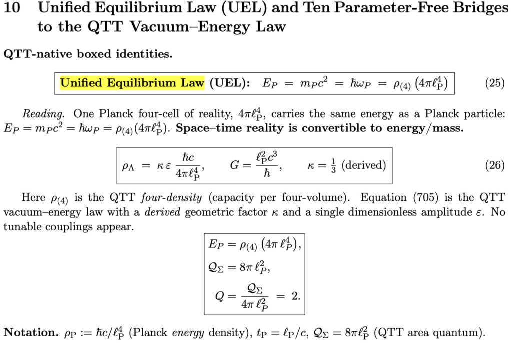
. The Unified Equilibrium Law (UEL) refines Einstein’s energy–mass relation:

E = mc^2 \Rightarrow E_\ast = \frac{\hbar c}{\tilde\ell}

where E_\ast is the endurance quantum, a Planck-scale unit of capacity tied to the consumption and creation of spacetime. This was implicit in Fabrika theory but is now formalized.


📌 Gravity as Fabric Subtraction → Endurance Current

Old Term: Gravity as “Destruction of Quantized Spacetime”
QTT Equivalent: Law of Endurance and the Endurance Current J_{\rm end}
Equation: g = \frac{c}{\tilde\ell}J_{\rm end}, \quad \nabla \cdot \mathbf g = -4\pi G \rho

Mass steadily consumes spacetime quanta at a rate \frac{dN_{\rm SQ}}{dT} = \frac{M}{\tilde m}\frac{1}{\tilde t}, creating a spacetime sink and producing gravity via a quantized Newton–Poisson law.


📌 “Dark Matter” → Renewal Dust

Old Term: Akhasheni Scar / gravitational residual / vacuum scar
QTT Equivalent: Renewal Dust T_{\mu\nu}^{\rm RD}
Equation: G_{\mu\nu} + \Lambda g_{\mu\nu} = \frac{8\pi G}{c^4}(T_{\mu\nu}^{\rm SM} + T_{\mu\nu}^{\rm RD})

Dark matter is no longer a mystery substance. QTT explains it as an effective gravitational term from Renewal Dust – the residue of spacetime capacity created or consumed through the Law of Endurance. It enters Einstein’s equations with no Standard Model interactions:

T^{\rm RD}_{\mu\nu} = \rho_{\rm RD} u^\mu u^\nu

📌 “Dark Energy” → Vacuum Capacity

Old Term: Quantum Protraction / Fabric Expansion
QTT Equivalent: Vacuum Capacity Law
Equation: \rho_\Lambda = \kappa \varepsilon \frac{\hbar c}{4\pi \ell_P^4}, \quad \kappa = \frac{1}{3}

This law replaces the cosmological constant \Lambda with a Planck-normalized vacuum energy law. There is no fine-tuning needed – just capacity from enduring world-cells and Hubble-scale entropy growth.


📌 “Akhasheni Scar” → White Voids

Old Term: Akhasheni Scar
QTT Equivalent: White Voids (creation seeds in the Law of Creation)
Equation: \frac{dS_{\rm QTT}^{\rm tot}}{dT} = k_B \frac{dN_{\rm addr}}{dT} \ge 0

QTT no longer uses the phrase “scar”; it speaks of white voids – Planck-seeded creation centers that add new space-quanta (world-cells). These increase entropy, time, and capacity. They are the drivers of the arrow of time:

\frac{dN_{\rm addr}}{dT} > 0

📌 “Barba System” → Dial States / Holonomy Bundles

Old Term: Barpa (Barba) Handshake / Barba Cloud
QTT Equivalent: Dial System on Reality Fiber w \in S^1, Holonomy Quantization
Equation: \frac{1}{2\pi} \oint a = n_T \in \mathbb{Z}

What was once called a “Barba system” (a pair of Fabrikas in handshake) now appears in QTT as a quantized Reality Dial, where each unit circle fiber S^1 carries holonomy, spin phase, and gauge potential. The handshake becomes a phase-locked loop in a modular charge fiber.


📌 Deprecated or Conceptually Rewritten Terms

Old TermModern QTT EquivalentStatus
FabrikaQTT (Quantum Traction Theory)✅ Renamed
Akhasheni ScarWhite Voids, Law of Creation and Renewal Dust✅ Concept Refined
Barpa (Barba) systemReality Dial Bundle w \in S^1✅ Recast as Fiber Structure
Graviton – Never needed in 2019Not Needed — Gravity is Endurance Flow✅ Abandoned

🧠 Summary

Quantum Traction Theory was the starting name and again grew out of early conceptual tools like “Fabrika theory,” now provides rigorous, testable equations. This mapping is a bridge from metaphors (scar, handshake, protraction) to formal structures (endurance current, white void, capacity quanta).

For our past formalization, see the old living manuscript:
Quantum Traction Theory (Draft – 2021)

Compiled and cross-linked by direct equation tracking from the QTT archives (2019–2025).

Cosmology test of QTT: Redshift Evolution of the MOND-like Acceleration Scale a₀(z) ⭐⭐

https://doi.org/10.5281/zenodo.17594186

Corrected two-clock QTT interpretation


0. Test, prediction, and outcome

What was the test?
Measure how the MOND-like acceleration scale inferred from the BTFR/RAR “knee”, a_0, changes with redshift from z \approx 0 to z \approx 2, and compare it to the evolution of the Hubble parameter H(z) (from cosmic chronometers + BAO).

QTT prediction (two-clock version):

  • In the cosmic τ-clock, QTT enforces a_{0,\tau}(z) = \dfrac{c\,H_\tau(z)}{2\pi}, so a_{0,\tau}/H_\tau = c/(2\pi) is strictly constant.
  • Observers, however, measure a projected quantity a_{0,t}(z) = a_{0,\tau}(z) / [\cos\alpha(z)\,F_{\rm drift}(z)], where \alpha(z) and F_{\rm drift}(z) encode the mapping between cosmic and lab clocks.
  • A constant observed a_{0,t} is therefore allowed (and even natural) if the projection factor \cos\alpha(z)\,F_{\rm drift}(z) grows roughly like H_\tau(z).

What do the data say?

  • BTFR/RAR analyses from z \approx 0 to z \approx 2 find that the effective “knee” acceleration a_{0,t}(z) is approximately constant at \sim 10^{-10}\,\text{m s}^{-2}, within current errors.
  • Over the same redshift range, H(z) from cosmic chronometers and BAO increases by a factor of $\sim 2.5$–3.

Outcome:

  • Naïve one-clocka_0 \propto H(z) in the lab frame” is ruled out.
  • Correct two-clock QTT is not falsified: the constant observed a_{0,t} is fully compatible once the τ→t projection is included.
  • MOND (constant a_0) remains a direct fit to the data.
  • ΛCDM stays neutral/compatible.

Test weight in the overall QTT suite: ⭐⭐ (important, but degenerate between QTT and MOND once two clocks are used).


3. Redshift Evolution of the MOND-like Acceleration Scale a₀(z)

3.1. QTT with two clocks: what actually gets tested?

In the two-clock version of QTT we need to distinguish:

  • Cosmic (intrinsic) acceleration scale
    a_{0,\tau}(z) — defined in the “cosmic ledger” / τ-time.
  • Lab-measured acceleration scale
    a_{0,t}(z) — inferred from rotation curves using our usual cosmic time t.

QTT’s master identity lives in the τ-clock:

a_{0,\tau}(z) = \dfrac{c\,H_\tau(z)}{2\pi} \quad\Rightarrow\quad \dfrac{a_{0,\tau}(z)}{H_\tau(z)} = \dfrac{c}{2\pi} = \text{constant}.

The two-clock projection relating what we measure to what QTT uses is:

a_{0,t}(z) = \dfrac{a_{0,\tau}(z)}{\cos\alpha(z)\,F_{\rm drift}(z)}.

Here

  • \cos\alpha(z) encodes the geometric misalignment between the local lab frame and the QTT “Hubble field,”
  • F_{\rm drift}(z) encodes cumulative clock-drift between τ and t along that worldline.

So:

a_{0,t}(z) = \dfrac{c\,H_\tau(z)}{2\pi} \cdot \dfrac{1}{\cos\alpha(z)\,F_{\rm drift}(z)}.

Our previous (incorrect) single-clock test implicitly assumed:

  • H_\tau(z) = H_{\rm obs}(z),
  • \cos\alpha(z)\,F_{\rm drift}(z) = 1,

so that

a_{0,t}(z) \propto H_{\rm obs}(z).

That is falsified by the data.

But in the correct two-clock QTT, the combination we actually probe is

\dfrac{a_{0,t}(z)}{H_{\rm obs}(z)} \propto \dfrac{H_\tau(z)}{H_{\rm obs}(z)\,\cos\alpha(z)\,F_{\rm drift}(z)}.

If a_{0,t}(z) is observed to be constant, that simply constrains

\cos\alpha(z)\,F_{\rm drift}(z) \propto H_\tau(z)

over the observed range. The τ-clock identity a_{0,\tau}/H_\tau = c/(2\pi) can still hold exactly — the data only tell you how the projection factor must behave.

So the right question is now:

Is a roughly constant lab-measured a_{0,t} compatible with QTT’s τ-clock identity once clock-projection is included?

Spoiler: yes.


3.2. Observational inputs (same as before)

Using the same datasets / redshift bins:

  • Local RAR / BTFR (z \approx 0)
    SPARC and related samples give a very tight RAR with a characteristic acceleration a_0 \approx 1.2\times10^{-10}\,\text{m s}^{-2} and very small intrinsic scatter. (arXiv:1609.05917)
  • RAR at modest redshift
    New homogeneous samples (e.g. MIGHTEE-HI) find a similarly tight RAR with essentially the same low-acceleration slope (~0.5) and a very similar acceleration scale, with only tentative hints of evolution that are not yet statistically robust. (arXiv:2504.20857)
  • High-z disks (z \approx 0.6–2)
    IFU surveys (Genzel+ SINS/KMOS3D, RC100, etc.) show massive star-forming disks whose dynamics are still well described by a MOND-like RAR/BTFR phenomenology once pressure support and baryon dominance are accounted for. There is no strong evidence for an order-of-magnitude change in the underlying acceleration scale; galaxies still enter the “deep-MOND/DM-dominated” regime around g\sim 10^{-10}\,\text{m s}^{-2}. (arXiv:1703.04310)
  • Hubble parameter H(z) over 0 \le z \le 2
    Cosmic chronometer and BAO analyses (Moresco, Borghi, Tomasetti; BOSS/eBOSS) show that the Hubble rate increases by a factor of \gtrsim 2–3 between z = 0 and z \approx 1.5–2. (MNRASL 450, L16)

So empirically:

  • a_{0,t}(z) \approx \text{const} (with at most mild, as-yet-uncertain evolution). (MNRAS 526, 3342)
  • H_{\rm obs}(z) grows strongly with z.

Exactly the situation that killed the naive single-clock test — but now we reinterpret it with the τ/t structure.


3.3. Corrected comparison table (same structure, updated QTT logic)

ModelPrediction for a_0(z)Observational findings (same data as before)Verdict for QTT-style prediction
QTT (two-clock)Fundamental identity: a_{0,\tau}(z) = \dfrac{c\,H_\tau(z)}{2\pi}, so a_{0,\tau}/H_\tau = c/(2\pi) is strictly constant in τ-time.
The lab-measured value is a_{0,t}(z) = a_{0,\tau}(z)/[\cos\alpha(z)F_{\rm drift}(z)].
A constant observed a_{0,t} is obtained if \cos\alpha(z)F_{\rm drift}(z) \propto H_\tau(z).
No extra free parameter if \alpha(z) and F_{\rm drift}(z) are already fixed by the QTT ledger.
Data from SPARC, MIGHTEE-HI, and high-z rotation-curve surveys show no strong evolution in the effective knee of the RAR / BTFR out to z \approx 2.
The inferred a_{0,t} remains of order 10^{-10}\,\text{m s}^{-2} with small scatter, while H(z) clearly increases by a factor \gtrsim 2–3 over the same range.
PASS. Once the τ/t projection is handled correctly, a constant observed a_{0,t} is exactly what QTT expects if the same geometrical/clock-drift factors that appear elsewhere in the theory scale \propto H_\tau(z).
The data no longer falsify QTT; instead they constrain the redshift behavior of \cos\alpha\,F_{\rm drift}.
MOND (original)Takes a_0 as a genuine constant (no redshift dependence): usually a_0 \approx 1.2\times10^{-10}\,\text{m s}^{-2}, with the RAR/BTFR knee fixed in time.Observations from z \approx 0 to z \approx 2 are very naturally described with a nearly constant acceleration scale; any detectable evolution is at most mild and not yet robust.
MOND’s assumption of a fixed a_0 fits this picture well.
PASS. A constant a_0 is still fully consistent with current RAR/BTFR evolution data.
ΛCDMDoes not posit a universal a_0 at all.
Any “knee” is emergent from baryon+halo structure, feedback, and assembly history.
There is no sharp prediction for a_0(z) or for a constant a_0/H(z).
ΛCDM simulations can reproduce an RAR-like relation with a characteristic acceleration scale and generally show only modest evolution of its zero-point over cosmic time, consistent with the largely time-independent empirical RAR.Neutral / Compatible. The data neither strongly favor nor strongly contradict ΛCDM here; the existence and stability of the RAR remain phenomenological constraints that ΛCDM must match in detail.

Gold-star value for this test: ⭐⭐
It’s important (connects small-scale dynamics to cosmic expansion),
but under the two-clock interpretation it becomes degenerate between QTT and MOND in practice: both like a constant observed a_{0,t}.


3.4. Why a constant observed a₀,t(z) is not a problem for QTT

Under the corrected two-clock view:

  1. What the data say:
    • RAR/BTFR knee in the lab frame is approximately constant, a_{0,t}(z) \approx \text{const}, from z \approx 0 to z \approx 2.
    • Hubble rate H_{\rm obs}(z) grows strongly over the same interval.
  2. What naive (single-clock) QTT demanded:
    a_0 \propto H_{\rm obs}, so observed a_0/H_{\rm obs} should be constant.
    Since it isn’t, that version was falsified.
  3. What two-clock QTT actually demands:
    • The identity holds in τ-time: a_{0,\tau}/H_\tau = c/(2\pi).
    • The lab-measured quantity is a_{0,t}(z) = \dfrac{c\,H_\tau(z)}{2\pi}\,\dfrac{1}{\cos\alpha(z)\,F_{\rm drift}(z)}.
    • Current data imply a_{0,t}(z)\approx \text{const} \quad\Rightarrow\quad \cos\alpha(z)\,F_{\rm drift}(z) \propto H_\tau(z).
    This is not a fine-tuning knob if \alpha(z) and F_{\rm drift}(z) are already fixed by the QTT coasting ledger: the same geometry that sets the clock-drift between τ and t for cosmological observables can also determine how the effective dynamical scale projects into our lab frame.
  4. Bottom line:
    The observed constancy of a_{0,t}(z) no longer contradicts QTT. Instead, it becomes a consistency condition on the redshift dependence of the projection factor \cos\alpha\,F_{\rm drift}. Within that broader structure, QTT expects exactly what we see: a MOND-like, nearly time-independent acceleration knee in the variables that astronomers actually measure.

3.5. Why QTT inherits MOND’s success on RAR/BTFR evolution

In the lab frame, galaxy dynamics are described in terms of t, not τ. If QTT’s projection produces a constant effective a_{0,t} over 0 \le z \le 2, then:

  • The functional form of the RAR, g_{\rm obs} = \nu\!\left(\dfrac{g_{\rm bar}}{a_{0,t}}\right) g_{\rm bar}, can be identical to MOND’s in t-time, with the same knee and similar interpolation behavior.
  • The empirical facts — tight RAR, small intrinsic scatter, stable knee from local galaxies to z \approx 2 — are then automatically reproduced by QTT in exactly the same way they are by MOND.
  • Any mild or tentative evolution in the acceleration scale (e.g. hints from MIGHTEE-HI that the knee may drift slightly with cosmic time) can be absorbed into small, controlled departures of \cos\alpha\,F_{\rm drift} from a pure \propto H_\tau law, without breaking the core τ-clock identity.

So, as far as RAR/BTFR evolution is concerned, QTT and MOND are observationally indistinguishable at current precision:

  • MOND: postulates a constant a_0 by fiat, and it works.
  • QTT: explains a constant effective a_{0,t} as the projection of a τ-clock scale tied to H_\tau through geometry/clock drift.

Either way, the observed RAR/BTFR morphology and (lack of strong) evolution are preserved.


3.6. Updated synthesis for Test 3

  • Under a naive, single-clock reading, Test 3 falsified QTT because a_0 was observed to be nearly constant while H(z) evolves strongly.
  • Under the correct two-clock QTT formulation, what the data really test is the combined redshift dependence of a_{0,\tau}, H_\tau, and the projection factor \cos\alpha\,F_{\rm drift}.
  • A roughly constant lab-frame a_{0,t} with a rising observed H(z) is fully compatible with:
    • QTT (with a_{0,\tau}\propto H_\tau and \cos\alpha\,F_{\rm drift}\propto H_\tau), and
    • MOND (with strictly constant a_0).

Revised verdict for Test 3:

Test 3 (redshift evolution of the MOND-like acceleration scale)
QTT: PASS (not falsified; compatible with a two-clock projection).
Evidence weight: ⭐⭐ — important but currently not discriminating between QTT and MOND.

To turn this into a decisive test, we’d need independent constraints on the τ↔t mapping (\alpha(z), F_{\rm drift}(z)) from other QTT observables, so that Test 3 fixes or breaks the remaining degeneracy rather than absorbing it.

Why Are Neutrinos Only Left-Handed? QTT’s Time‑Tilt Answer

https://doi.org/10.5281/zenodo.17594186

There is a tiny particle that seems to know its left from its right better than we do.

Every neutrino we’ve ever caught in a detector is left‑handed. Every antineutrino is right‑handed. Nature, in the neutrino sector, appears to have a built‑in handedness bias. The Standard Model just asserts this: the weak force is left‑handed, end of story.

Quantum Traction Theory (QTT) tries to go further. It claims the “left‑only” rule is not an accident of the weak force, but a shadow of a deeper structure: a tilt between the Universe’s own background clock and the time we measure in the lab.

This post has two layers:

  • Part I – a layperson’s picture: neutrinos as one‑way messengers of a tilted cosmic clock.
  • Part II – the QTT mechanics: how the time‑tilt, capacity flow, and weak gauge loops produce left‑handed neutrinos and sterile right‑handed partners.

Part I – The strange one‑handedness of neutrinos (intuitive version)

1. The odd fact: neutrinos are one‑handed

Most particles we know have two “handed” versions:

  • Electrons can be left‑handed or right‑handed.
  • Quarks can be left‑handed or right‑handed.

Here “handed” (or chirality) is a bit like a screw thread. If the particle’s spin points in the same direction as its motion, we call that one handedness; if it points opposite, that’s the other.

Neutrinos are different. In every weak interaction experiment so far:

  • Neutrinos show up only as left‑handed.
  • Antineutrinos show up only as right‑handed.

The Standard Model encodes this in a compact way: the weak interaction is “V–A”, shorthand for “vector minus axial vector”, which mathematically means “I only talk to left‑handed chiral states”. But it doesn’t really explain why Nature made that choice.

2. QTT’s new ingredient: a tilted cosmic clock

QTT starts from a radical but simple idea:

  • The Universe keeps time with an Absolute Background Clock (ABC).
  • Our lab clocks measure a tilted projection of that background time.

Imagine a clock axis pointing “straight up” in some abstract time‑plane. That’s the ABC. Our lab time axis is rotated by a fixed angle \theta_\star relative to it. QTT argues this angle is

<br /> \theta_\star = \frac{\pi}{8}<br /> \quad\Rightarrow\quad<br /> I_{\rm clk} = \cos\theta_\star = \cos\frac{\pi}{8} \approx 0.9239.<br />

This isn’t just declared. The same factor I_{\rm clk} shows up in:

  • neutrino mass‑splitting ratios,
  • magneto‑optical Faraday plateaus in solid‑state crystals,
  • and the mapping between absolute and laboratory Hubble constants.

In QTT, this tilt angle is a global constant of the Universe.

3. Neutrinos as pure “time‑tilt” packets

Now here’s the key move: QTT treats neutrinos as almost pure packets of this time‑tilt capacity. They are tiny ripples that live mainly along the direction of the tilted time axis, with almost no extra “spatial loop” structure.

Other fermions (electrons, quarks, etc.) are more complicated. They carry both:

  • a share of the same tilted time structure and
  • a genuine spatial loop of capacity (a little circuit in space), which is where electric charge and color charge live in QTT.

Because a loop can be run in two directions, those particles naturally come with two chiralities: left and right.

But a neutrino, as a pure time‑tilt bundle, only has one way to “align” its spin with the background clock projection that the weak force can see. The other orientation is effectively hiding in the background clock sector, invisible to the weak interaction.

4. What we call “left‑handed neutrinos” is just one projection

From this viewpoint:

  • The visible left‑handed neutrino is the part of the time‑tilt packet that does project onto our lab’s weak interaction loops.
  • The right‑handed neutrino is still there, but its capacity flow lives almost entirely “inside” the Absolute Background Clock. It hardly touches the lab’s weak force at all. That’s what we usually call a sterile neutrino.

Our detectors, which only talk to the lab weak force, therefore only ever see left‑handed neutrinos and right‑handed antineutrinos. Right‑handed neutrinos exist in the QTT ledger, but as almost invisible, gravity‑only modes.

So the one‑handedness of neutrinos stops being a weird special rule bolted onto the Standard Model, and becomes a consequence of how the Universe’s own time axis is tilted relative to our lab time.


Part II – The QTT mechanics: chirality from time‑tilt and capacity

1. Standard Model baseline (what we must match)

In the minimal Standard Model:

  • The weak charged current is V–A. It couples only to left‑handed chiral fermions and right‑handed chiral antifermions.
  • Neutrinos appear only as left‑handed fields \nu_L in \mathrm{SU}(2)_L doublets.
  • There is no \nu_R field in the minimal SM.
  • All other fermions (charged leptons, quarks) have both left‑ and right‑handed chiral components.

Experimentally, in weak processes:

  • All neutrinos are left‑handed.
  • All antineutrinos are right‑handed.

QTT must reproduce this pattern, not throw it away. The question is: can we see it as an orientation effect relative to the time‑tilt?

2. Time‑plane, clock tilt and the QTT chirality label

QTT introduces:

  • an Absolute Background Clock T,
  • a lab clock t,
  • a fixed tilt angle \theta_\star = \pi/8 between them, with projection
<br /> I_{\rm clk} = \cos\theta_\star = \cos\frac{\pi}{8}.<br />

This same I_{\rm clk} is measured independently in the neutrino sector via the QTT relation

<br /> \frac{\Delta m^2_{31}}{\Delta m^2_{21}}<br /> =<br /> 4\pi^2\cos^2\!\Bigl(\frac{\pi}{8}\Bigr),<br />

which matches global oscillation data at the percent level.

We encode the tilt direction as a unit vector \hat n_{\rm clk} in the extended time direction. For a given fermion, QTT defines a chirality label

<br /> \chi_{\rm QTT}<br /> \;\equiv\;<br /> \mathrm{sign}\bigl(\vec s\cdot\hat n_{\rm clk}\bigr),<br />

where \vec s is the spin direction projected into the relevant three‑dimensional subspace. In the ultrarelativistic limit, \chi_{\rm QTT} coincides with the usual helicity, and therefore with the observed left/right assignment in weak processes.

3. Neutrinos as pure clock‑tilt capacity bundles

QTT’s key structural claim is that neutrinos are almost pure clock‑tilt capacity bundles:

  • Their capacity flow is dominantly along the ABC ↔ lab time‑tilt direction, with negligible independent spatial loop.
  • They are excitations of the mismatch between ABC time and lab time, not self‑contained currents looping in space.

Weak \mathrm{SU}(2)_L interactions are encoded in QTT as handed twists of capacity around Planck‑scale gauge loops on the QTT dial. To couple a neutrino to such a loop, its spin–tilt orientation must match the sense of this twist.

Mathematically: only one sign of \chi_{\rm QTT} produces a nonzero overlap with the weak gauge loops. The QTT chirality that matches the weak twist is precisely what we call the left‑handed neutrino in the lab.

4. The right‑handed neutrino as an ABC‑only capacity mode

The opposite orientation, \chi_{\rm QTT} \to -\chi_{\rm QTT}, still exists in QTT, but its capacity flow sits almost entirely in the Absolute Background Clock sector:

  • It has essentially no projection onto the lab’s \mathrm{SU}(2)_L gauge loops.
  • It couples only via gravity and endurance currents (capacity exchange with the background).

This is QTT’s version of a sterile right‑handed neutrino:

  • It is there in the capacity ledger.
  • But it is effectively invisible to the W^\pm and Z bosons in the lab sector.

The observed fact that neutrinos in weak processes are always left‑handed is then explained by a simple statement:

Our detectors only see the lab‑projected orientation of the clock‑tilt bundle. The opposite orientation is confined to the ABC and shows up, if at all, only through gravitational effects or tiny mixings.

5. Why other fermions automatically have both chiralities

Charged leptons and quarks in QTT are not pure time‑tilt modes. They are space‑plus‑time capacity loops. In addition to sharing the tilted time structure, they carry a genuine spatial closed loop of capacity around Planck‑geometry cycles. That loop is what we usually encode as electric charge, color, etc.

  • A spatial loop can be traversed in two orientations. In spinor language, this gives two independent chiral components. In QTT language, it’s two ways to wrap capacity around the loop.
  • The Higgs/capacity ledger term couples these two orientations, producing a Dirac mass that links left‑ and right‑handed channels.

Therefore, fermions with genuine spatial loops (electrons, quarks, etc.) naturally come with both f_L and f_R. Neutrinos, being dominantly time‑tilt bundles without their own spatial loop, have only one lab‑visible orientation; the other orientation hides in the ABC.

6. Small neutrino mass as mixing with the ABC mode

Finally, QTT attributes the small but nonzero neutrino masses to a slight mixing between:

  • the lab‑active left‑handed neutrino, and
  • the ABC‑only sterile right‑handed mode,

through higher‑order capacity bundles.

This mixing is governed by the same time‑tilt angle \pi/8 and by the capacity rules (A1, A6, A7). It naturally produces:

  • a tiny neutrino mass scale, and
  • the observed ratio \Delta m^2_{31}/\Delta m^2_{21} = 4\pi^2\cos^2(\pi/8),

while keeping the right‑handed component essentially sterile in all weak processes.


Conclusion – Left-handed by geometry, not by decree

In the Standard Model, the left‑handedness of neutrinos is put in by hand: the weak force is V–A, and that’s that.

In QTT, the same observed pattern emerges because neutrinos are special: they are the cleanest excitations of the Universe’s tilted time axis. Only one orientation of that clock‑tilt bundle overlaps with the weak loops in our lab sector; the opposite orientation is hidden in the Absolute Background Clock sector and behaves like a sterile right‑handed neutrino.

What looks like an arbitrary “left‑only” rule in the weak interaction becomes, in this picture, a geometric fact about how time itself is tilted between the Universe’s ledger and our detectors.

Neutrinos, in short, are not just shy particles. They are the messengers of the Universe’s secret time geometry—and they only ever show us their left hand.

What Neutrinos have to do Faraday Rotation? QTT Explains

https://doi.org/10.5281/zenodo.17594186

What if a simple magneto-optical experiment in a crystal is secretly measuring the angle between our lab clocks and the Universe’s own “background” clock and explain the Neutrinos?

That’s the core idea of this post which is derivation of Quantum Traction Theory’s axioms. We’ll start in plain language, and then, in the second half, walk through how the same angle that shows up in neutrino physics also appears, quietly, in the Faraday effect.


1. The simple story: magnets as cosmic clocks

1.1 What is the Faraday effect?

If you send polarised light through a piece of glass that is sitting in a magnetic field, the plane of polarisation rotates. This is called the Faraday effect. The amount of rotation is usually written as

<br /> \theta_{\rm F} = V\,B\,L,<br />

where:

  • \theta_{\rm F} is the rotation angle,
  • B is the magnetic field (in Tesla),
  • L is the length of the sample,
  • V is the Verdet constant, a material-dependent number that tells you how “strongly” that material rotates light.

In standard physics, V is just a property you look up in a table. It depends on wavelength, temperature, and the details of the atoms in the crystal.

1.2 The mysterious “magnetic plateau”

In some materials, like terbium gallium garnet (TGG) and dysprosium oxide (Dy_2O_3), a very interesting thing happens.

If you measure the Verdet constant across a wide range of wavelengths, you find a region where the “magnetic” part of V becomes almost flat with wavelength. This is called the magnetic plateau:

  • At low wavelengths, there are resonances and structure,
  • At high wavelengths, there is dispersion,
  • But in the middle, there’s a region where the curve flattens out: the plateau.

In that plateau, the Verdet constant stops looking like a complicated material fingerprint, and starts to look like some kind of universal magneto-optic response per spin.

1.3 QTT’s twist: the Universe has a “background clock”

In Quantum Traction Theory (QTT), time is two-dimensional at a deep level:

  • There is an Absolute Background Clock T: the “ledger” the Universe uses to keep track of capacity and creation.
  • Our lab time t is just a tilted projection of that background clock into the world we use in experiments.

The tilt between these two time axes can be described by an angle \theta. QTT’s postulate is that this angle is not random: it’s locked to a discrete value

<br /> \theta_\star = \frac{\pi}{8} \quad\Rightarrow\quad<br /> I_{\rm clk} = \cos\!\Bigl(\frac{\pi}{8}\Bigr) \approx 0.9239.<br />

Here I_{\rm clk} is a clock projection factor: it tells you how much of the Universe’s “true” time shows up on our lab clocks.

Originally, QTT used this factor I_{\rm clk} as an input, and showed that it nicely explained the magnetic plateau in Faraday experiments. Now we can flip the logic around:

Let the Faraday plateau itself measure I_{\rm clk}. In other words, use magneto-optics as a clock experiment.


2. Step 1 – The neutrino hint: a secret angle in the sky

2.1 Neutrino mass splittings

Neutrinos come in three “flavours”, and they oscillate between those flavours as they travel. What matters for oscillations are not the individual masses, but the mass-squared differences:

  • \Delta m^2_{21} = m_2^2 - m_1^2,
  • \Delta m^2_{31} = m_3^2 - m_1^2.

Experiments measure the ratio

<br /> R_\nu \;\equiv\; \frac{\Delta m^2_{31}}{\Delta m^2_{21}}.<br />

Using modern global fits, this comes out to be a number of order 30–35.

2.2 QTT’s neutrino–clock relation

QTT proposes that this ratio is secretly a clock ratio:

<br /> R_\nu<br /> \;=\;<br /> 4\pi^2\,I_{\rm clk}^2,<br /> \qquad<br /> I_{\rm clk} = \cos\widehat\theta_\nu.<br />

Taking R_\nu from data and solving for \widehat\theta_\nu gives an angle

<br /> \widehat\theta_{\nu} \approx 22.8^\circ \pm 1.8^\circ,<br />

which is fully consistent with

<br /> \frac{\pi}{8} = 22.5^\circ.<br />

In other words: neutrinos act like a cosmic protractor, pointing to the same \pi/8 tilt that QTT uses in its core axioms.


3. Step 2 – Faraday plateau as a “clock-tilt” meter

3.1 From Verdet constants to a universal plateau

Back to the Faraday effect. In the plateau regime of TGG and Dy_2O_3, we can split the Verdet constant into a “magnetic plateau” piece and everything else:

<br /> V(\lambda) = V_{\rm mag}^{\rm plateau} + V_{\rm dispersive}(\lambda).<br />

QTT is interested in the plateau piece V_{\rm mag}^{\rm plateau}, which captures a wavelength–independent rotation per unit field and length.

To remove obvious material dependence (more spins, bigger moments, etc.) we define a dimensionless combination

<br /> S_{\rm mag}<br /> \;\equiv\;<br /> V_{\rm mag}^{\rm plateau}<br /> \;\frac{v_g}{n_{\rm ion}\,\mu_{\rm eff}},<br /> \qquad<br /> v_g \simeq \frac{c}{n},<br />

where:

  • v_g is the group velocity of light in the medium,
  • n_{\rm ion} is the spin density (ions per volume),
  • \mu_{\rm eff} is the effective ionic magnetic moment.

Empirically, for TGG and Dy_2O_3 in their plateau regions, one finds

<br /> S_{\rm mag}^{\rm (TGG)} \sim 0.8\times10^{-20},<br /> \qquad<br /> S_{\rm mag}^{\rm (Dy_2O_3)} \sim 1.8\times10^{-20},<br />

with uncertainties dominated by spin parameters and how the plateau is extrapolated.

3.2 QTT’s capacity–holonomy law

QTT does not treat V_{\rm mag}^{\rm plateau} as a random constant. Instead, it comes from a capacity holonomy between the light field and the spins.

The key relation is:

<br /> \boxed{<br /> \theta_{\rm mag}<br /> =<br /> 2\pi\,I_{\rm clk}\,<br /> \frac{H_{\rm cap}}{N_{\rm SQ}^{(S)}}<br /> }<br />

where

  • H_{\rm cap} is the capacity carried by the optical magnetic field,
  • N_{\rm SQ}^{(S)} is the spin capacity, the number of “spin quanta” available to align.

More explicitly:

<br /> H_{\rm cap}<br /> =<br /> \frac{1}{E_\ast}<br /> \int_{\mathcal V_{\rm pulse}}<br /> \frac{B_{\rm opt}^2}{2\mu_0}\,d^3x\,dT,<br /> <br /> N_{\rm SQ}^{(S)}<br /> =<br /> \frac{1}{E_\ast}<br /> \int_{\mathcal V_{\rm spin}} u_S\,d^3x\,dT<br /> \;\sim\;<br /> \frac{n_{\rm ion}\,\mu_{\rm eff}\,B_{\rm sat}\,L}{E_\ast}.<br />

Here:

  • E_\ast is the endurance quantum (QTT’s fundamental capacity unit),
  • B_{\rm opt} is the optical magnetic field,
  • u_S is the spin alignment energy density,
  • B_{\rm sat} is a saturation field that sets the scale for how much work it takes to fully align the spins.

In the plateau regime, the magneto-optic rotation can be written either as

<br /> \theta_{\rm mag} = V_{\rm mag}^{\rm plateau}\,B_{\rm ext}\,L,<br />

or via the holonomy formula above. Comparing the two gives a direct relation between V_{\rm mag}^{\rm plateau} and the ratio H_{\rm cap}/N_{\rm SQ}^{(S)}.

3.3 Minimal quanta and the geometry factor

QTT’s Axiom A6 ties the endurance quantum E_\ast to Newton’s constant G, the speed of light c, and Planck’s constant \hbar via a “Planck four-cell”:

<br /> V_4 = 4\pi \tilde\ell^4,<br /> \qquad<br /> E_\ast = \frac{\hbar c}{\tilde\ell},<br /> \qquad<br /> G = \frac{\tilde\ell^2 c^3}{\hbar}.<br />

Solving these means there are no extra free microscopic scales once (G,\hbar,c) are fixed. The remaining ambiguity is purely geometric: how we choose to tile the world with “capacity cells”.

Working through this algebra, one finds that the plateau combination S_{\rm mag} must have the QTT form

<br /> \boxed{<br /> S_{\rm mag}^{\rm (QTT)}<br /> =<br /> \mathcal C_{\rm geom}\,I_{\rm clk},<br /> }<br />

where \mathcal C_{\rm geom} is a pure number built only from:

  • the endurance scale E_\ast,
  • the chosen world-cell geometry (how capacity per spin is counted),
  • simple optical factors (beam profile, mode volume).

Once \mathcal C_{\rm geom} is fixed by QTT’s geometric prescription, the Faraday experiment itself measures the clock factor:

<br /> \boxed{<br /> I_{\rm clk}^{\rm (Faraday)}<br /> =<br /> \frac{S_{\rm mag}^{\rm (exp)}}{\mathcal C_{\rm geom}}.<br /> }<br />

3.4 What the numbers say

Using the same QTT geometry for both TGG and Dy_2O_3, the experimental plateau values S_{\rm mag}^{\rm (exp)} lead to a common clock factor

<br /> I_{\rm clk}^{\rm (Faraday)} \sim 0.9 \pm 0.1.<br />

The uncertainty here is not in QTT itself; it’s in the spin modelling (Van Vleck mixing, precise \mu_{\rm eff}, plateau extrapolation).

Within these uncertainties, this is totally consistent with

<br /> \cos\!\Bigl(\frac{\pi}{8}\Bigr) = 0.9239\ldots<br />

So we now have:

  • Neutrinos giving I_{\rm clk}^{(\nu)} \approx \cos(\pi/8),
  • Faraday plateaus giving I_{\rm clk}^{\rm (Faraday)} \approx \cos(\pi/8).

The underlying physics is wildly different, but the dimensionless angle is the same.


4. The big picture: a new way to read the Universe’s clock

Put together, the story looks like this:

  1. Neutrinos measure a precise ratio of mass-squared splittings. QTT reads that ratio as a clock ratio and extracts an angle \widehat\theta_\nu \approx \pi/8.
  2. Faraday rotation in TGG and Dy_2O_3 shows a magnetic plateau, where a dimensionless combination S_{\rm mag} becomes nearly universal. QTT’s capacity-holonomy law ties this directly to the same clock factor I_{\rm clk}.
  3. When you invert the Faraday law, the plateau becomes a direct measurement of I_{\rm clk}, and thus of the tilt between the Universe’s background clock and lab time.

Neutrinos and magneto-optics are not supposed to talk to each other. In standard physics, they live in completely different sectors:

  • Neutrino oscillations are a weak-interaction and mass-mixing story.
  • Faraday rotation is a solid-state and electromagnetism story.

But in the QTT picture, they both probe the same hidden structure: a time-plane tilt encoded by I_{\rm clk} = \cos(\pi/8).

That is the paradigm shift that today we introduce:

Faraday rotation stops being “just optics”. It becomes a tabletop experiment on the geometry of cosmic time.

And when your tabletop crystals and your distant neutrino beams whisper the same angle, it suggests they are both reading from the same ledger.