Foundations of Fabrika Physics
chapter 1-1 By: Ali Attar
: Abstract and history of Theory
Back in 1996, when I was in high school, my physics teacher Dr Ghasemi, said a couple of things that intrigued me deeply.
First one, was after he taught us about General Relativity and how precise it is in predictions related to the Gravity and gravitational lensing. However, it kind of breaks, by returning “infinity” when we are discussing black holes curvatures of Space/Time.
The second discussion was about unification of forces. And how gravity left alone and scientists are looking deeply to find a theory of everything to unify 4 forces and they haven’t been successful so far.
In that time, we always had fun, trying to solve the puzzles in our break time. However, these new puzzles, were so interesting for me, that I started to dive deeper into the problems of matching of General Relativity and Quantum Mechanics, almost everyday I have had quite thought experiments for the past 25 years to find solid answers to those puzzles that he seeded in my mind.
Over time, the theory that I developed, shaped better and seemed more and more logical to myself. It showed to me, rather than trying to connect General Relativity and Quantum Mechanics I should search for a fundamental underlaying theory to cover both. I focused my efforts, mainly to describe gravity first. To me, that was the starting point for most of the unanswered questions.
I found not only answers to those questions, but with the same theory, I found very solid and yet intuitive answers to lot of other physic mysteries like “Why and how matter creates curvature in space/time?”, “Does Dark Matter exist?”, “What is Dark Energy?”, “Why Hubble constant changed over time?”.
Back in 2019, one beautiful day in April, I was in Fabrika. A place in Tbilisi that usually young entrepreneurs and intellectuals are gathering, reading books and discussing ideas and sometimes get drunk!
In that day and in that moment in Fabrika, finally, I decided to talk about this deep though experiments after couple of decades! I named it Fabrika Theory in aspiration of that place that I made that decision. The name that I selected, stroke me after a while, when I realized, actually, the first chapter should be re-defining the “Fabrics” of Space/Time!
So I gathered a group of people, for the first time, to hear my theory and give me feedbacks. A physics professor in Georgia-Tbilisi, and 2 other physics enthusiasts. We started recording some YouTubE videos
https://www.youtube.com/channel/UCEPrRMy89i6kiVfIGud7cIQ about the theory and then discussed it and challenged my idea mostly off the camera. They questioned the theory as I expected, and I gave the answers one by one. It was a great couple of months journey.
During those meetings, the idea shaped even better. I made some more changes in the theory to make sure, we address the concerns of Professor specially.
In the next couple of years, while I was following my software business, (which has nothing to do with Physics) I worked more with 3 – 4 more physic experts to question the idea further, and shape it even better.
In these discussions, most of the people that I worked (and they had professional physics related teaching jobs, or research) emphasized a lot about not naming them as my advisors in this theory! Found out, that mainstream physics community is not very open to a new physics or a theory that can be an improvements to G.R. Or Q.M.
One of my advisors, told me, you will have a long way, for anyone to consider Fabrika theory as General Relativity and Quantum Mechanics are considered sacred and untouchable in the scientific community. Brutal truth? I hope not. I believe there is a difference between 16th century Church and 21st century’s scientific community.
If you are from this community, you need to have a very open mind, to continue reading this theory.
Fabrika theory, is not going to question any of experimental evidences of General Relativity or Quantum Mechanics. Rather, it tries to create more fundamental definitions that actually, predicts almost similar outcomes, specially in General Relativity, however for a totally different reasonings.
Foundations of Fabrika Physics
chapter 1-2 Definition of Fabrika Pixels
chapter 1-2 : Definition of Fabrika Pixels and Space-Time-Reality (STR).
Basis of Fabrika Physics starts with a new fundamental definition for Space Time and its nature.
Fabrika theory suggests that Space and Time is NOT a continuum like what is suggested in General Relativity (ref:
https://einstein.stanford.edu/content/relativity/q411.html ) and this will result to certain predictions, specially about Dark Matter and Gravity that over the next chapters, we will discuss.
Fabrika Theory also suggest, there is another dimension that I name it ”Reality Dimension” and it has different properties than Space dimensions and Time dimension. (Chapter 1-3). So from now, we will call Space-time as Space-Time-Reality (STR).
The definition of Fabrika Pixels is a little challenging as it has no precedent in modern or classic physics.
First, we start what Fabrika Pixel is NOT:
Single Fabrika pixels are not particles or virtual particles
Single Fabrika pixels are not holding information
Single Fabrika pixels are not type of force or field
And Fabrika Pixels have certain properties and features:
They represent one blank length in all space dimensions.
They “rotate” in certain direction. This is not like normal rotation or spin, it’s a hypothetical term, for property of Single Fabrika Pixels. This rotation creates the “time forward” and also “asymmetry” in certain upcoming predictions of Fabrika theory.
Single Fabrika Pixels (SFPs), are responsible for existence of Space-time-Reality and universe in whole.
They can have handshake with each other and that will be “information” or “matter” or “energy” . These handshakes, they can convert to other type of handshakes. (E.g. conversation of mass to energy and vice versa) . Hand-shaking Fabrika Pixels (HFPs) are creating Barba systems (Chapter 1-5 )
In “single” state they can be destructed. (Redefining Gravity – Chapter 2-1).
When as Single state , they recreate themselves in a constant rate. (Introduction of new constant = SFPs creation rate). This is their (Single Fabrika Pixels) natural property . (Vacuum Energy will be calculated based on this and Dark Energy mystery will be addressed by equation related to this. Also cosmological constant in General relativity will be defined here.) (Expansion of Space-Time-Reality – Chapter 2-2)
Foundations of Fabrika Physics
chapter 1-3: Reality Dimension
(Will add in the next editions)
Foundations of Fabrika Physics
chapter 1-4: Handshaking Fabrika Pixels
(Will add in the next editions)
Foundations of Fabrika Physics
chapter 1-5: Barba Systems
(Will add in the next editions)
Fabrika Gravity
chapter 2-1 Redefining Gravity – Introduction
Introduction: One of the most essential predictions of Fabrika Theory, is about Gravity and how it works. In Fabrika theory, I have defined a very simple and intuitive cause for Gravity which falls in line with the predictions of two famous theories in short distances:
Newton Theory of gravity (Chapter 2-2)
Einstein Theory of General relativity
And falls in line with
prediction of MOND in larger scales.
About gravitational lensing the theory falls in line with the reductions of:
General Relativity
And predicts a theory of the called “Akhasheni Scars” to explain the mysteries of “gravitational lensing” without presence of related mass. (Or gravitational field) in certain cases like bullet clusters.
The formula, has a pretty simple foundation:
Matter continuously destructs Single Fabrika Pixels and that’s the root cause of gravity:
As Single Fabrika Pixels are representing Time/Space/Reality, the effect of Gravity happens
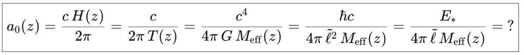
The acceleration and “force” that we feel as gravity is based on the number of Single Fabrika pixels destructed per second. This aligns with the Newton Formula of Gravity. “G” will be recalculated based on the new constant (Constant 2) that will be introduce by Fabrika theory.
The “curvature” in “space-time” happens by continues destruction of Single Fabrika pixels by matter, and therefore, all of the predictions of General Relativity in short distances will be applicable. In longer distances, Fabrika theory will return different results which doesn’t need dark matter to account for gravity.
Fabrika Gravity Principal: The gravity will act different in distances by the following reasons:
1. Plank Size of Gravity Calculation (Destruction of Single Fabrika Pixels) which results to have not possibility of dividing the Gravity effect further (minimum is plank size) in very far distances. It can’t go smaller than a certain value because of Plank size (General Relativity allows that because you can divide the gravity to infinity). To understand better, the exact same thing happens to be the answer in Ultraviolet catastrophe!! Now, we found it in Gravity.
and 2. Nature of Gravity in Fabrika gravity. Nature of Gravity is destruction of SFPs. This means, in a galaxy system for example, the total destructed numbers of SFPs will be equal by the mass of the galaxy! and therefore, the gravity effect will be more in compare to the curvature of space time presented by General Relativity.
So if calculated acceleration by gravity effect, is less than a certain number (I like to refer to MOND Gravity) because distance is MORE than a certain number, Gravity in Fabrika theory will not be splittable anymore, (Plank size minimum effect)
Fabrika Gravity / Quantum Traction
chapter 2-2 Matching with Newton Gravity
Matching Fabrika Gravity with Newton’s Gravity was my very first step of validating the theory of Fabrika.
After all, Newton Gravity had the simplest definition for Gravity for a long time and if I wanted to make sure, that Gravity is working as I am thinking, it suppose to match with Newton Gravity at least in simplest systems. (Apple – Earth!)
The thought experiment was totally successful and destruction of Single Fabrika Pixels by matter could replicate the effects of Gravity predicted as a “force” by Newton.
Basically, how I imagined it was simple. Destruction of Single Fabrika Pixels by matter can be imagined as a Sphere that creates traction and pulling other SFPs from the universe around it in every direction. I called this quantized effect of gravity “Quantum Traction” and I named my youtube channel and website after it. This definitely has nothing to existing definitions of quantum mechanics.
This means, the number of Fabrikas going down toward the massive Sphere from the universe, is proportional to the surface of that sphere and it’s related directly to the mass that sphere has. This idea has the following results:
Each body of mass, will have the gravity effect totally independent from the second body of mass. In Newtonian gravity, you will need two body of mass to calculate the gravity. In Fabrika theory, one body of mass, is enough to calculate the SFPs destructed per second.
The outcome of calculation is pretty match with Newton Gravity.
The speed of replacement of destructed SFPs with provided SFPs from universe is equal to C and that’s how effect of gravity travels with the speed of light in every direction. However, what is defining G is *number* of SFPs destructed per second / maximum that can be destructed per second. To understand this better, consider a sq-meter surface which has the gravity pulling. (for example 1 sq meter of surface of earth). A certain number of Fabrikas are passing toward center of earth. A limited number and the wave that they create is “Gravity”. If we have a number equal by 1meter divided to plank size, power by 2, we are talking about Surface of event horizon of Blackhole.
The acceleration that each objects gets is depend on how many Fabrikas are passing with the speed of light through them. (For example per square centimeter). This creates an outcome acceleration which we know as gravitational “force” in Newtonian gravity. For example in earth we reach to the 9.8/ms2 like Newtonian gravity.
Another example,In the event horizon of Blackhole, all of available SFPs in the surface are moving by the speed of light for replacing the destructed Single Fabrika Pixels in Blackhole.
…….
Akhasheni Scars
Chapter 2 – 3 : Where space/time/reality deformed
Abstract:
Based on part of the Fabrika theory, the continues destructions of Fabrikas, creates deformation of space/time/reality. During the time, this deformation or scar will be deeper and it can cause gravitational lensing without even presenting the related matter.
There is a an analogy for this. Consider a monitor, showing same static picture for a month. Basically, pixels on this monitor, will be burned to the same color that they were showing during that month. Now, if you turn off the monitor, or change the picture, the hallo of original picture is still there!
Or consider, a scar on your face. Even if all of the cells and molecules of your skin change over years, the scar remains there. so deformation of Space / Time and Reality gets deepen.
This prediction happens in Fabrika theory to explains why scientists in the past 70 years, have been very confused by “gravitational lensing”. In Fabrika theory (in contradiction with General Relativity” which predicts only case 1) Gravitational lensing happens for 2 different cases:
Case 1: By presence of matter (speed = c) = Fabrika Gravity = Destruction of SFPs >>> which causes curvature in space time and reality similar to prediction in General Relativity
Case 2 : By having the above effect “long enough” and interact with continues replacement of destructed SFPs by universe around the object and shaping “Akhasheni Scars” deeply in Space/Time/Reality. In this case OBSERVED GRAVITY EFFECT is always MORE than present matter. and this “More” is depend how old or young the evaluated galaxy and galaxy cluster is.
So Fabrika theory predicts, there can be gravitational lensing without presence of the related (or enough matter) if we move that matter after long time of destruction of SFPs. Deformation and scars will be remain there. Matter can move on. (Case 2)
Also Fabrika theory predicts, the Akhasheni scars can create extra “gravity curvature” without presence of related matter! This will create change how Galaxy Clusters move around each other in a very long period of time.

), the observed frequencies shift in a precise way:
Prediction: tightening or delaying the gate changes rates via
, residual tick-overlap causes small, quantitative deviations from the asymptotic frequency that vanish like
. (Space trials widely and the deviations disappear.)
that fixes subtle intensity ratios when the instrument is perfectly balanced. (This enters as a relative amplitude factor; flux normalization is preserved.)
where
shifts and overlaps the two gates by a delay
. Prediction: move the coincidence window and the joint frequencies follow this overlap law.
with an extra, measurable prefactor set by the gate-overlap variance. Tune gates → tune the prefactor; the Born limit itself remains the same.
follows the overlap law above and saturates to the standard Born weight as
.
amplitude ratio in carefully normalized branch intensities (with total flux conserved).


 .
.
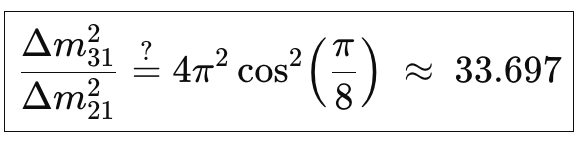
 : a prediction from Quantum Traction’s “two-clock” Artian geometry.
 .
. and the mass ordering.
 .
. or
or  .
.