
When the Dark Port Speaks
A receiver can cancel a source's phase. One detector equation shows how, why quantum mechanics agrees, and what would make the next experiment genuinely different.
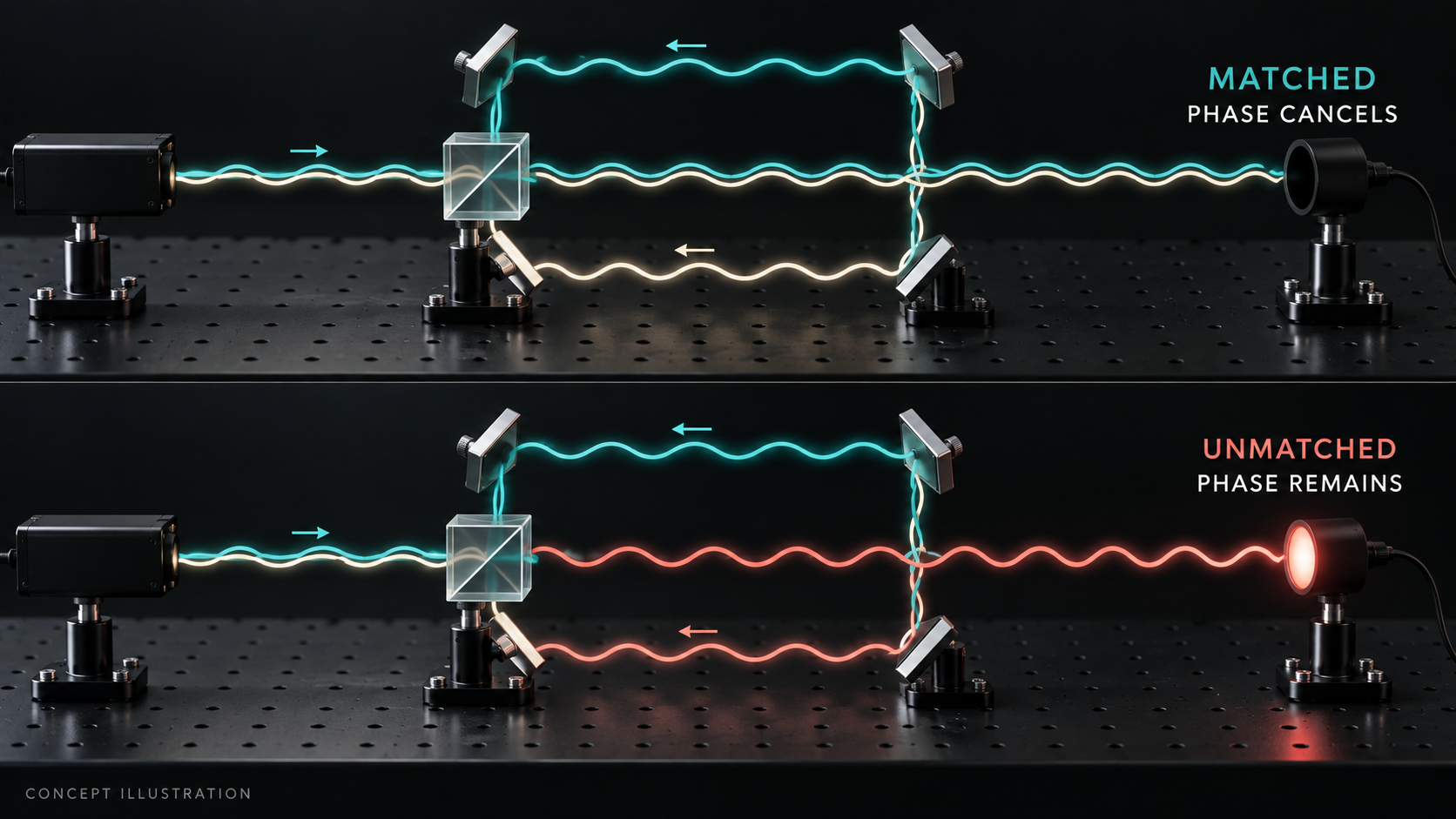
Imagine a detector that should be silent.
Two alternatives reach the same final comparison. One supplies a reference. The other carries a small sequence of operations: change an internal phase, shift an internal state, and undo those changes in the specified order. Although the internal carrier returns to its starting configuration up to phase, the sequence can leave a phase behind. When the alternatives meet, that phase can turn silence into clicks.
Now let the receiver participate. Give it the matching, oppositely oriented transport. The phase left by the source is cancelled by the receiver. The detector goes dark again.
In the completed-event construction, that statement becomes a short equation:

The left side is a detector probability. The right side contains the number of internal states and the weight of a precisely defined source-receiver matching sector. It turns a question about what a receiver has access to into something an experimentalist can count.
Here is the important distinction at the outset. For this specified apparatus, ordinary quantum mechanics gives exactly the same equation. QTT's opportunity lies in explaining and independently constraining the physical source and contact that produce it. A new-physics result would require a further, testable difference on the same apparatus. The equation tells us where to look; it does not manufacture that difference.
Field Notes · Quantum FoundationsWhat the detector is counting
The label dark names the output port that is dark when the loop acts as the identity. It does not promise that the port stays dark in every configuration.
The equation assumes a balanced, coherent comparison with an identity reference arm, an independently set reference phase, and ideal readout. Real beam-splitter imbalance, loss, detector bias and phase drift belong in the independently calibrated instrument model.
The integer d counts the internal states of the finite carrier. It is a specified physical encoding, not a number adjusted until the clicks look right. The quantity eta, written as the Greek letter in the equations, is the population of the qualified matching sector. Formally, M is its projector and rho is the prepared state:

This matching is more precise than lining up two optical paths. On that sector the receiver must implement the conjugate transport defined by the contact theorem. In the complementary sector of this particular model, it remains idle. A shared address, an attractive diagram, or the word "receiver" does not establish those operations.
For a three-state carrier, the result is particularly easy to read:
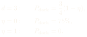
Those are calculated ideal limits, not reported experimental measurements. The intermediate value eta = 1/2 gives 37.5%. No extra coefficient is fitted to obtain any of them once the carrier, state and operations have been specified.
The striking feature is relational. The same source-side operation can leave a visible phase when the receiver is idle and no net phase when the receiver carries its qualified counterpart.
Field Notes · Quantum FoundationsFour operations leave one phase
Think of d positions arranged around a dial. One operation, Z, assigns successive phase marks to those positions. Another, V, advances the internal state by one position. Changing phase and then shifting is not the same as shifting and then changing phase. Their difference is one phase step around the dial.
This is the finite clock-shift algebra studied by Julian Schwinger in 1960. The QTT paper uses it inside an explicit source-receiver contact, rather than claiming that the algebra itself is new. In familiar complex notation, its loop identity is:
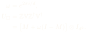
Products act from right to left. Fixing that order matters: reversing the loop reverses the signed phase. The bold operations act on the matching flag, source and receiver together. On the matched sector, the source's phase and the receiver's conjugate phase multiply to one. On the unmatched sector, the source phase remains.
The loop is a scalar phase within each sector. Such a phase becomes measurable through comparison with the coherent reference alternative; it is not measurable merely by looking at an isolated carrier.
The interferometer reads the loop amplitude L. The familiar controlled-unitary readout of a trace is described, for example, by Ekert and colleagues. Here the trace and the detector probability are:
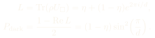
The last step uses the elementary identity 1 - cos(2x) = 2 sin squared(x). It is a detector-level consequence of the paper's finite-loop theorem, not an additional axiom.
For a reader new to QTT, the paper's imaginary unit has an upstream account: a real orientation operator J with J squared equal to minus the identity. Writing i here makes the laboratory calculation familiar; it does not withdraw that real-source construction. The finite phase step is fixed by the specified d-state representation. A1 supplies completed-event ordering in this use, not an extra numerical phase factor.
Field Notes · Quantum FoundationsWhy ordinary quantum mechanics reappears
It is tempting to say that QTT "usually collapses to QM." That mixes two different ideas.
First, this is not wavefunction collapse. We are comparing descriptions. Second, for the states and operations just written, the agreement is exact throughout the allowed parameter range, including intermediate matching. There is no hidden threshold where changing eta automatically makes ordinary QM stop working.
The same is true of the paper's Bell reconstruction. A real-source geometry, qualified composition rule, neutral pair and quadratic capacity readout lead to the familiar correlation formulas. After phase alignment, with g the magnitude of the retained record overlap, two useful Bell expressions are:

The first uses the specified 45-degree settings; the second optimizes the settings for that correlation tensor. They are not interchangeable. The Bell overlap g is also not the loop population eta. The paper provides no permission to identify them just because both lie between zero and one.
Why should a different ontology recover familiar mathematics? Because a source theory must account for the reliable phenomena already described by quantum mechanics. QTT's construction attempts to explain the source structure behind that successful description: which real orientations compose, what a completed contact retains, and how retained capacity becomes a detector frequency under a stated frequency bridge.
That is a substantive reconstruction under explicit premises. It is not, by itself, an experiment choosing QTT over QM. For these specified circuits, neither calculation needs an extra coefficient fitted to the target counts. Both require the state, contact operations and instrument calibration. The comparison must credit that equally.
Field Notes · Quantum FoundationsTwo meanings of the Access Law
The broad Access-Law question is already present: what part of a source becomes a retained laboratory record through this particular contact? A detector does not report an unmediated source description. It reports the result of a physical interaction and a chosen readout.
Conventional quantum measurement theory also has source states, instruments and retained records. The stronger QTT task is to derive which contact maps are physically available from its finite source ontology, rather than treating every laboratory-relevant map as an unconstrained input. The present paper constructs a definite contact class and supplies finite probes that can qualify its matching condition.
There is also a more specific Access uncertainty relation in the corpus. In conventional notation, a qualified matched/unmatched quadrature model has:
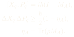
The subscript A is deliberate. M_A is a quadrature matching projector; it is not automatically the finite-loop projector M. The equality between their physical meanings would need a contact theorem, not a change of notation.
For the declared operators, state domain and finite moments, the uncertainty bound follows from the commutator. At eta_A = 0, it has the familiar canonical lower bound. At eta_A = 1, this particular lower bound is zero. That does not force zero fluctuations, guarantee a state attaining the bound, or prove that an ordinary particle's canonical position and momentum can be jointly measured with arbitrary precision.
There is a useful historical check. Ordinary two-system quantum mechanics already permits a relative position and a total momentum to commute:

That distinction belongs to the Einstein-Podolsky-Rosen discussion of 1935. Commuting joint observables are not a violation of the canonical relation for one constituent. A proposed Access-Law experiment must identify the actual observables before interpreting an unusual uncertainty product.
Nor does a finite loop silently prove an exact canonical commutator. The trace of a finite matrix commutator is zero, whereas the trace of a nonzero constant times the identity is not. Passing from a finite carrier to continuum quadratures requires its own representation and domain argument. The paper keeps those constructions separate.
Field Notes · Quantum FoundationsWhere new physics could enter
The decisive question is not whether a detector clicks at the value above. A deliberately implemented controlled loop already has that answer in ordinary QM. The decisive question is whether QTT can independently specify a real material contact and restrict its response in a way that a matched physical comparator does not predict.
There are three distinct scientific outcomes.
A reconstructed description. QTT and QM assign the same state, operations and readout probabilities. The result establishes a correspondence and makes the proposed source ontology concrete. It is not an empirical separation.
A new source prediction within quantum behavior. QTT derives a contact parameter or allowed structure that an effective quantum model previously took from measurement. A held-out success can favor that source explanation even when the resulting dynamics remain quantum-mechanical. Deriving a previously supplied input is valuable without calling it a violation of QM.
A genuinely different laboratory prediction. QTT's independently fixed contact law and an independently specified conventional matter-and-instrument model predict different distributions for the same physical experiment. A controlled, reproducible result can then discriminate between them. Disagreeing with one effective model would first reject that model; a claim about quantum mechanics more broadly needs a correspondingly broader argument.
These possibilities do not require a theory to become arbitrary at the boundary of its correspondence. They require the missing physical identification to become more precise.
For this paper, the next task is to derive the receiver's matching behavior from the independently specified contact dynamics. That includes determining whether the loop projector, the quadrature projector and the Bell overlap share a physical relation. We cannot assume that relation and then count its consequences as three independent confirmations.
Field Notes · Quantum FoundationsThe experiment worth doing
A serious experiment would start with the contact, not with a target probability on the screen.
- Specify the physical degrees of freedom. State what the d internal states, matching flag, source and receiver are in the apparatus, and which interaction implements each operation. Fix their meaning before examining the outcome data.
- Qualify the matching independently. Use the theorem's basis and superposition probes, with simultaneous uncertainty bounds, to test the receiver's conjugate transport. Estimate the prepared matching population without deriving it backwards from the dark-port count being tested.
- Measure a phase scan and reverse the loop. The full interference response retains the signed phase. The single dark-port probability at zero reference phase does not distinguish the two loop orientations, because its cosine is even. A quadrature measurement or phase scan is therefore essential.
- Freeze both physical predictions. Print every independently calibrated quantity, free coefficient and discrete choice on both sides. If the two predictions coincide, call the experiment a construction test. If they differ, preregister the distribution-level discriminator, uncertainty budget and required precision.
- Keep the controls and the failures. Test path imbalance, phase offsets, drift, leakage and detection bias; retain rejected and unsuccessful outcomes under a declared counting rule. Validate on data not used to choose the contact law.
One practical consequence follows immediately. The sharp 0-to-75% ideal contrast at d = 3 makes the specified construction conspicuous. It does not supply a 75-percentage-point difference between QTT and QM. Statistical significance must be calculated for the actual difference between competing predictions, not for the existence of interference.
Field Notes · Quantum FoundationsWhat the existing record establishes
The paper already includes an independent replay of a public quantum-information archive: 40,032 stored tree records from 7,952 shots. The supplied success and failure scoring is reproduced. That checks the handling of the recorded outcomes; it does not mean every random outcome was predicted in advance.
The archive and its experimental publication test a different instrument from the proposed finite loop. The declared retrospective, job-cluster tests give nominal p-values of about 0.019 and 0.044 for the shared ideal-instrument predictions, with independent jobs assumed. Those residuals remain part of the audit. They are not a high-significance QTT-over-QM win, because the matched predictions there are identical.
The v2.0 paper contains the proof, probe qualifications, instrument model and replay. Its finite-contact results appear in Sections 11.1-11.4, especially the loop theorem and response on page 20. Its Access uncertainty discussion and scope are on pages 16-17; the archive execution is on pages 23-26. These are same-author derivation and reproducibility anchors, not independent experimental endorsements.
For a self-contained introduction to the record analysis, see the separate Record-Deletion Benchmark. It tests seven ways of hiding outcomes across all five primary-batch strengths, with complete reproduction materials. It uses overlapping data, not a second independent experiment.
Field Notes · Quantum FoundationsWhy this equation is worth keeping
The detector equation makes an abstract claim answerable. It says exactly what cancels, which receiver action cancels it, what remains when the receiver is idle, and how the difference reaches a countable record.
That is the contribution I find most interesting: the receiver becomes part of the physical explanation, not just the place where we put the final number. The mathematics is explicit enough to test a construction and precise enough to show what still separates that test from a test of new physics.
For students and researchers, QTT's proposed source ontology remains speculative physics. The conditional mathematical results can be checked now; this detector equation has not independently selected that ontology over ordinary quantum mechanics. The next advance would be a source-derived physical contact whose held-out consequences are no longer interchangeable with the competing account.
A dark detector can tell us something remarkable. First we have to establish exactly why it is dark.